4 Chapter 6: Designs with Variation in Treatment Timing
4.1 Overview
Dataset: Wolfers (2006) — wolfers2006_didtextbook.dta
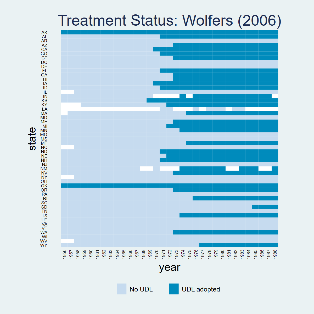
This chapter analyzes the effect of unilateral divorce laws (UDL) on divorce rates using a binary-and-staggered design. Between 1968 and 1988, 29 US states adopted UDLs. The panel covers 51 states from 1956 to 1988, with population weights and state-clustered standard errors throughout.
Key topics: decomposition of the static TWFE estimator, event-study TWFE, and four heterogeneity-robust estimators (Sun & Abraham, Callaway & Sant’Anna, de Chaisemartin & D’Haultfœuille, Borusyak et al.).
4.2 PanelView
* ssc install panelview, replace
copy "https://raw.githubusercontent.com/anzonyquispe/did_book/main/cc_xd_didtextbook_2025_9_30/Data%20sets/Wolfers%202006/wolfers2006_didtextbook.dta" "wolfers2006_didtextbook.dta", replace
use "wolfers2006_didtextbook.dta", clear
panelview div_rate udl, i(state) t(year) type(treat) title("Treatment Status: Wolfers (2006)") legend(label(1 "No UDL") label(2 "UDL adopted"))library(panelView)
load(url("https://raw.githubusercontent.com/anzonyquispe/did_book/main/cc_xd_didtextbook_2025_9_30/Data%20sets/Wolfers%202006/wolfers2006_didtextbook.RData"))
png("figures/ch06_panelview_R.png", width = 1000, height = 600)
panelview(div_rate ~ udl, data = df, index = c("state", "year"), type = "treat",
main = "Wolfers (2006)", ylab = "")
dev.off()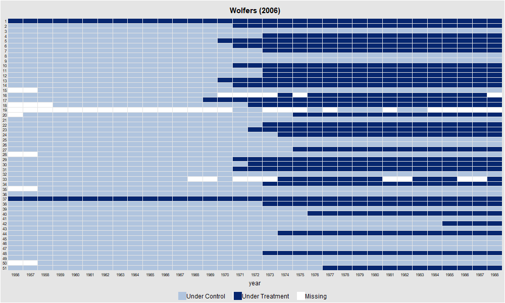
import pandas as pd
import matplotlib.pyplot as plt
import matplotlib.colors as mcolors
from matplotlib.patches import Patch
df = pd.read_parquet("https://raw.githubusercontent.com/anzonyquispe/did_book/main/cc_xd_didtextbook_2025_9_30/Data%20sets/Wolfers%202006/wolfers2006_didtextbook.parquet")
states_sorted = (df.groupby("state")["cohort"]
.first().sort_values(ascending=False).index)
state_idx = {s: i for i, s in enumerate(states_sorted)}
years = sorted(df["year"].unique())
fig, ax = plt.subplots(figsize=(14, 10))
cmap = mcolors.ListedColormap(["#4292C6", "#EF6548"])
for _, row in df.iterrows():
si = state_idx[row["state"]]
yi = years.index(row["year"])
color = 1 if row["udl"] == 1 else 0
ax.add_patch(plt.Rectangle((yi, si), 1, 1, color=cmap(color)))
ax.set_xlim(0, len(years)); ax.set_ylim(0, len(states_sorted))
ax.set_xticks(range(0, len(years), 5))
ax.set_xticklabels([str(int(years[i])) for i in range(0, len(years), 5)],
rotation=45, fontsize=7)
ax.set_yticks([i + 0.5 for i in range(len(states_sorted))])
ax.set_yticklabels(states_sorted, fontsize=6)
ax.set_xlabel("Year"); ax.set_ylabel("State")
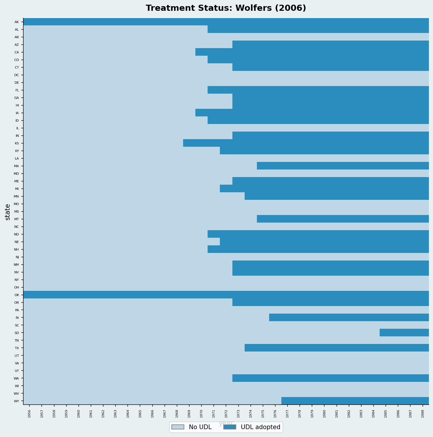
ax.set_title("Treatment Status: Wolfers (2006)")
legend_elements = [Patch(facecolor="#4292C6", label="Control"),
Patch(facecolor="#EF6548", label="Treated")]
ax.legend(handles=legend_elements, loc="lower right")
plt.tight_layout()
plt.savefig(FIGDIR / "ch06_panelview_Python.png", dpi=150)4.3 CQ#25: Static TWFE Regression
Run the static TWFE regression of
div_rateon state and year FEs and the UDL treatment, weighting by population and clustering at the state level. Do UDLs have an effect on divorces?
copy "https://raw.githubusercontent.com/anzonyquispe/did_book/main/cc_xd_didtextbook_2025_9_30/Data%20sets/Wolfers%202006/wolfers2006_didtextbook.dta" "wolfers2006_didtextbook.dta", replace
use "wolfers2006_didtextbook.dta", clear
reg div_rate udl i.state i.year [w=stpop], vce(cluster state)
Linear regression Number of obs = 1,631
R-squared = 0.9305
Root MSE = .52417
(Std. err. adjusted for 51 clusters in state)
------------------------------------------------------------------------------
| Robust
div_rate | Coefficient std. err. t P>|t| [95% conf. interval]
-------------+----------------------------------------------------------------
udl | -.0548378 .1507695 -0.36 0.718 -.3576673 .2479917
------------------------------------------------------------------------------library(haven); library(fixest)
load(url("https://raw.githubusercontent.com/anzonyquispe/did_book/main/cc_xd_didtextbook_2025_9_30/Data%20sets/Wolfers%202006/wolfers2006_didtextbook.RData"))
m1 <- feols(div_rate ~ udl + i(year) | state,
data = df, weights = ~stpop, cluster = ~state,
ssc = ssc(fixef.K = "full"))Variable Coefficient Std. err. t [95% Conf. Interval]
------------------------------------------------------------------------------------------
udl -0.0548378 0.1507695 -0.36 [ -0.3503461, 0.2406705]
N = 1631 | R-sq = 0.9305import pandas as pd
import pyfixest as pf
df = pd.read_parquet("https://raw.githubusercontent.com/anzonyquispe/did_book/main/cc_xd_didtextbook_2025_9_30/Data%20sets/Wolfers%202006/wolfers2006_didtextbook.parquet")
m1 = pf.feols('div_rate ~ udl + i(year) | state',
data=df, weights='stpop', vcov={'CRV1': 'state'},
ssc=pf.ssc(adj=True, fixef_k='full', cluster_adj=True))Variable Coefficient Std. err. t [95% Conf. Interval]
------------------------------------------------------------------------------------------
udl -0.0548378 0.1507695 -0.36 [ -0.3503461, 0.2406705]
N = 1631 | R-sq = 0.9305Interpretation: \(\hat{\beta}_{fe} = -0.055\) (s.e. = 0.15, p = 0.72). The coefficient is small and insignificant — according to this regression, UDLs do not affect divorce rates.
4.4 CQ#26: Decompose Static TWFE
Decompose \(\hat{\beta}_{fe}\) using
twowayfeweights. Does it estimate a convex combination of effects? Could it be biased for the ATT?
* ssc install twowayfeweights, replace
copy "https://raw.githubusercontent.com/anzonyquispe/did_book/main/cc_xd_didtextbook_2025_9_30/Data%20sets/Wolfers%202006/wolfers2006_didtextbook.dta" "wolfers2006_didtextbook.dta", replace
use "wolfers2006_didtextbook.dta", clear
twowayfeweights div_rate state year udl, type(feTR) test_random_weights(exposurelength) weight(stpop)
Under the common trends assumption,
the TWFE coefficient beta, equal to -0.0548, estimates a weighted sum of 522 ATTs.
490 ATTs receive a positive weight, and 32 receive a negative weight.
------------------------------------------------
Treat. var: udl # ATTs Σ weights
------------------------------------------------
Positive weights 490 1.0259
Negative weights 32 -0.0259
------------------------------------------------
Total 522 1.0000
------------------------------------------------
Regression of variables possibly correlated with the treatment effect on the weights
Coef SE t-stat Correlation
exposurele~h -8.2883613 .21360588 -38.80212 -.73253245library(haven); library(TwoWayFEWeights)
load(url("https://raw.githubusercontent.com/anzonyquispe/did_book/main/cc_xd_didtextbook_2025_9_30/Data%20sets/Wolfers%202006/wolfers2006_didtextbook.RData"))
decomp2 <- twowayfeweights(df, "div_rate", "state", "year", "udl",
type = "feTR",
test_random_weights = "exposurelength",
weights = df$stpop)Under the common trends assumption,
beta estimates a weighted sum of 522 ATTs.
490 ATTs receive a positive weight, and 32 receive a negative weight.
Treat. var: udl ATTs Σ weights
Positive weights 490 1.0259
Negative weights 32 -0.0259
Total 522 1
Regression:
Coef SE t-stat Correlation
RW_exposurelength -8.288361 0.2136059 -38.80212 -0.7325324import pandas as pd
from twowayfeweights import twowayfeweights
df = pd.read_parquet("https://raw.githubusercontent.com/anzonyquispe/did_book/main/cc_xd_didtextbook_2025_9_30/Data%20sets/Wolfers%202006/wolfers2006_didtextbook.parquet")
result = twowayfeweights(df, "div_rate", "state", "year", "udl",
type="feTR", weights="stpop",
test_random_weights="exposurelength")Under the common trends assumption,
beta estimates a weighted sum of 522 ATTs.
490 ATTs receive a positive weight, and 32 receive a negative weight.
Sum of positive weights: 1.0259
Sum of negative weights: -0.0259
Regression of variables possibly correlated with the treatment effect on the weights
Coef SE t-stat Correlation
exposurelength -8.288361 0.213606 -38.8021 -0.732532Interpretation: Under parallel trends, \(\hat{\beta}_{fe}\) estimates a weighted sum of ATTs. The vast majority receive positive weights (sum ≈ 1.026) and 32 receive negative weights (sum ≈ −0.026) — an “almost convex” combination. However, weights are strongly negatively correlated with exposure length (corr = −0.73, t = −38.8): \(\hat{\beta}_{fe}\) heavily downweights long-run effects. It could differ from the ATT if treatment effects vary with length of exposure.
4.5 CQ#27: Test Randomized Treatment Timing
Test whether pre-treatment outcomes differ across early, late, and never adopters (excluding always-treated states, restricting to years ≤ 1968).
copy "https://raw.githubusercontent.com/anzonyquispe/did_book/main/cc_xd_didtextbook_2025_9_30/Data%20sets/Wolfers%202006/wolfers2006_didtextbook.dta" "wolfers2006_didtextbook.dta", replace
use "wolfers2006_didtextbook.dta", clear
reg div_rate i.early_late_never if cohort!=1956 & year<=1968 [w=stpop], vce(cluster state)
Linear regression Number of obs = 611
F(2, 47) = 7.46
Prob > F = 0.0015
R-squared = 0.1707
(Std. err. adjusted for 48 clusters in state)
----------------------------------------------------------------------------------
| Robust
div_rate | Coefficient std. err. t P>|t| [95% conf. interval]
-----------------+----------------------------------------------------------------
early_late_never |
2 | -.0457088 .4927483 -0.09 0.926 -1.03699 .9455728
3 | -1.363398 .3751166 -3.63 0.001 -2.118035 -.608761
|
_cons | 3.054891 .2584305 11.82 0.000 2.534996 3.574786
----------------------------------------------------------------------------------library(haven)
load(url("https://raw.githubusercontent.com/anzonyquispe/did_book/main/cc_xd_didtextbook_2025_9_30/Data%20sets/Wolfers%202006/wolfers2006_didtextbook.RData"))
df3 <- df %>% filter(cohort != 1956, year <= 1968)
m3 <- feols(div_rate ~ i(early_late_never),
data = df3, weights = ~stpop, cluster = ~state,
ssc = ssc(fixef.K = "full"))Variable Coefficient Std. err. t [95% Conf. Interval]
------------------------------------------------------------------------------------------
(Intercept) 3.0548909 0.2584305 11.82 [ 2.5483670, 3.5614147]
early_late_never::2 -0.0457088 0.4927483 -0.09 [ -1.0114954, 0.9200777]
early_late_never::3 -1.3633981 0.3751166 -3.63 [ -2.0986266, -0.6281697]
N = 611 | R-sq = 0.1707import pandas as pd
df = pd.read_parquet("https://raw.githubusercontent.com/anzonyquispe/did_book/main/cc_xd_didtextbook_2025_9_30/Data%20sets/Wolfers%202006/wolfers2006_didtextbook.parquet")
df3 = df[(df['cohort'] != 1956) & (df['year'] <= 1968)].copy()
m3 = pf.feols('div_rate ~ C(early_late_never)',
data=df3, weights='stpop', vcov={'CRV1': 'state'},
ssc=pf.ssc(adj=True, fixef_k='full', cluster_adj=True))Variable Coefficient Std. err. t [95% Conf. Interval]
------------------------------------------------------------------------------------------
Intercept 3.0548909 0.2584305 11.82 [ 2.5483670, 3.5614147]
C(early_late_never)[T.2.0] -0.0457088 0.4927483 -0.09 [ -1.0114954, 0.9200777]
C(early_late_never)[T.3.0] -1.3633981 0.3751166 -3.63 [ -2.0986266, -0.6281697]
N = 611 | R-sq = 0.1707Interpretation: F-test p-value = 0.0015 — we reject that pre-treatment outcomes are the same across groups. Treatment timing is not randomly assigned: never-adopters have significantly lower divorce rates before any state adopts a UDL.
4.6 CQ#28: Event-Study TWFE Regression
Run the event-study TWFE regression with
rel_timeindicators. Test pre-trends jointly.
copy "https://raw.githubusercontent.com/anzonyquispe/did_book/main/cc_xd_didtextbook_2025_9_30/Data%20sets/Wolfers%202006/wolfers2006_didtextbook.dta" "wolfers2006_didtextbook.dta", replace
use "wolfers2006_didtextbook.dta", clear
reg div_rate rel_time* i.state i.year [w=stpop], vce(cluster state)
test rel_timeminus1-rel_timeminus9
(Std. err. adjusted for 51 clusters in state)
--------------------------------------------------------------------------------
| Robust
div_rate | Coefficient std. err. t P>|t| [95% conf. interval]
---------------+----------------------------------------------------------------
rel_time1 | .2891561 .2054259 1.41 0.165 -.1234539 .7017661
rel_time2 | .3358503 .1024966 3.28 0.002 .1299798 .5417208
rel_time3 | .3037197 .0958368 3.17 0.003 .1112258 .4962136
rel_time4 | .2162947 .1100871 1.96 0.055 -.0048218 .4374112
rel_time5 | .1824478 .1135503 1.61 0.114 -.0456248 .4105203
rel_time6 | .2469589 .1235802 2.00 0.051 -.0012592 .4951769
rel_time7 | .2521922 .1354015 1.86 0.068 -.0197698 .5241541
rel_time8 | .1684823 .1324744 1.27 0.209 -.0976004 .434565
rel_time9 | -.007686 .1224421 -0.06 0.950 -.2536183 .2382463
rel_time10 | -.1312296 .135582 -0.97 0.338 -.4035541 .1410948
rel_time11 | -.1795675 .1618587 -1.11 0.273 -.5046704 .1455353
rel_time12 | -.3662379 .165442 -2.21 0.031 -.698538 -.0339379
rel_time13 | -.3894262 .1685244 -2.31 0.025 -.7279175 -.0509349
rel_time14 | -.4421197 .1949527 -2.27 0.028 -.8336937 -.0505457
rel_time15 | -.3402803 .1710816 -1.99 0.052 -.6839078 .0033472
rel_time16 | -.526895 .2602054 -2.02 0.048 -1.049533 -.0042572
rel_timeminus1 | .0401147 .0525088 0.76 0.448 -.0653522 .1455817
rel_timeminus2 | .0377587 .058556 0.64 0.522 -.0798546 .1553719
rel_timeminus3 | .0997316 .0674681 1.48 0.146 -.0357821 .2352453
rel_timeminus4 | .0988424 .0897758 1.10 0.276 -.0814777 .2791625
rel_timeminus5 | .020862 .1099841 0.19 0.850 -.2000476 .2417716
rel_timeminus6 | .0183927 .1151678 0.16 0.874 -.2129287 .2497141
rel_timeminus7 | .0602846 .1119554 0.54 0.593 -.1645845 .2851537
rel_timeminus8 | .0808726 .1471298 0.55 0.585 -.2146462 .3763915
rel_timeminus9 | .0558855 .1600016 0.35 0.728 -.2654871 .3772581
---------------+----------------------------------------------------------------
F( 9, 50) = 0.51
Prob > F = 0.8631library(haven)
load(url("https://raw.githubusercontent.com/anzonyquispe/did_book/main/cc_xd_didtextbook_2025_9_30/Data%20sets/Wolfers%202006/wolfers2006_didtextbook.RData"))
rt_vars <- c(paste0("rel_time", 1:16), paste0("rel_timeminus", 1:9))
rt_formula <- as.formula(paste("div_rate ~", paste(rt_vars, collapse = " + "),
"+ i(year) | state"))
m4 <- feols(rt_formula, data = df, weights = ~stpop, cluster = ~state,
ssc = ssc(fixef.K = "full"))
wald(m4, keep = paste0("rel_timeminus", 1:9))Variable Coefficient Std. err. t [95% Conf. Interval]
------------------------------------------------------------------------------------------
rel_time1 0.2891561 0.2054259 1.41 [ -0.1134786, 0.6917908]
rel_time2 0.3358503 0.1024966 3.28 [ 0.1349569, 0.5367437]
rel_time3 0.3037197 0.0958368 3.17 [ 0.1158795, 0.4915599]
rel_time4 0.2162947 0.1100871 1.96 [ 0.0005240, 0.4320654]
rel_time5 0.1824478 0.1135503 1.61 [ -0.0401109, 0.4050064]
rel_time6 0.2469589 0.1235802 2.00 [ 0.0047418, 0.4891760]
rel_time7 0.2521922 0.1354015 1.86 [ -0.0131948, 0.5175791]
rel_time8 0.1684823 0.1324744 1.27 [ -0.0911675, 0.4281321]
rel_time9 -0.0076860 0.1224421 -0.06 [ -0.2476726, 0.2323006]
rel_time10 -0.1312296 0.1355820 -0.97 [ -0.3969703, 0.1345111]
rel_time11 -0.1795675 0.1618587 -1.11 [ -0.4968107, 0.1376756]
rel_time12 -0.3662379 0.1654420 -2.21 [ -0.6905043, -0.0419716]
rel_time13 -0.3894262 0.1685244 -2.31 [ -0.7197342, -0.0591183]
rel_time14 -0.4421197 0.1949527 -2.27 [ -0.8242270, -0.0600124]
rel_time15 -0.3402803 0.1710816 -1.99 [ -0.6756002, -0.0049604]
rel_time16 -0.5268950 0.2602054 -2.02 [ -1.0368975, -0.0168925]
rel_timeminus1 0.0401147 0.0525088 0.76 [ -0.0628025, 0.1430319]
rel_timeminus2 0.0377587 0.0585560 0.64 [ -0.0770112, 0.1525285]
rel_timeminus3 0.0997316 0.0674681 1.48 [ -0.0325059, 0.2319691]
rel_timeminus4 0.0988424 0.0897758 1.10 [ -0.0771182, 0.2748030]
rel_timeminus5 0.0208620 0.1099841 0.19 [ -0.1947069, 0.2364309]
rel_timeminus6 0.0183927 0.1151678 0.16 [ -0.2073362, 0.2441217]
rel_timeminus7 0.0602846 0.1119554 0.54 [ -0.1591481, 0.2797173]
rel_timeminus8 0.0808726 0.1471298 0.55 [ -0.2075017, 0.3692470]
rel_timeminus9 0.0558855 0.1600016 0.35 [ -0.2577175, 0.3694885]
N = 1631 | R-sq = 0.9351
Wald test: stat = 0.506103, p-value = 0.870968, on 9 and 1,523 DoFimport pandas as pd
df = pd.read_parquet("https://raw.githubusercontent.com/anzonyquispe/did_book/main/cc_xd_didtextbook_2025_9_30/Data%20sets/Wolfers%202006/wolfers2006_didtextbook.parquet")
rt_pos = [c for c in df.columns if c.startswith("rel_time") and "minus" not in c]
rt_neg = [c for c in df.columns if "rel_timeminus" in c]
fml = "div_rate ~ " + " + ".join(rt_pos + rt_neg) + " + i(year) | state"
m4 = pf.feols(fml, data=df, weights='stpop', vcov={'CRV1': 'state'},
ssc=pf.ssc(adj=True, fixef_k='full', cluster_adj=True))Variable Coefficient Std. err. t [95% Conf. Interval]
------------------------------------------------------------------------------------------
rel_time1 0.2891561 0.2054259 1.41 [ -0.1134786, 0.6917908]
rel_time2 0.3358503 0.1024966 3.28 [ 0.1349569, 0.5367437]
rel_time3 0.3037197 0.0958368 3.17 [ 0.1158795, 0.4915599]
rel_time4 0.2162947 0.1100871 1.96 [ 0.0005240, 0.4320654]
rel_time5 0.1824478 0.1135503 1.61 [ -0.0401109, 0.4050064]
rel_time6 0.2469589 0.1235802 2.00 [ 0.0047418, 0.4891760]
rel_time7 0.2521922 0.1354015 1.86 [ -0.0131948, 0.5175791]
rel_time8 0.1684823 0.1324744 1.27 [ -0.0911675, 0.4281321]
rel_time9 -0.0076860 0.1224421 -0.06 [ -0.2476726, 0.2323006]
rel_time10 -0.1312296 0.1355820 -0.97 [ -0.3969703, 0.1345111]
rel_time11 -0.1795675 0.1618587 -1.11 [ -0.4968107, 0.1376756]
rel_time12 -0.3662379 0.1654420 -2.21 [ -0.6905043, -0.0419716]
rel_time13 -0.3894262 0.1685244 -2.31 [ -0.7197342, -0.0591183]
rel_time14 -0.4421197 0.1949527 -2.27 [ -0.8242270, -0.0600124]
rel_time15 -0.3402803 0.1710816 -1.99 [ -0.6756002, -0.0049604]
rel_time16 -0.5268950 0.2602054 -2.02 [ -1.0368975, -0.0168925]
rel_timeminus1 0.0401147 0.0525088 0.76 [ -0.0628025, 0.1430319]
rel_timeminus2 0.0377587 0.0585560 0.64 [ -0.0770112, 0.1525285]
rel_timeminus3 0.0997316 0.0674681 1.48 [ -0.0325059, 0.2319691]
rel_timeminus4 0.0988424 0.0897758 1.10 [ -0.0771182, 0.2748030]
rel_timeminus5 0.0208620 0.1099841 0.19 [ -0.1947069, 0.2364309]
rel_timeminus6 0.0183927 0.1151678 0.16 [ -0.2073362, 0.2441217]
rel_timeminus7 0.0602846 0.1119554 0.54 [ -0.1591481, 0.2797173]
rel_timeminus8 0.0808726 0.1471298 0.55 [ -0.2075017, 0.3692470]
rel_timeminus9 0.0558855 0.1600016 0.35 [ -0.2577175, 0.3694885]
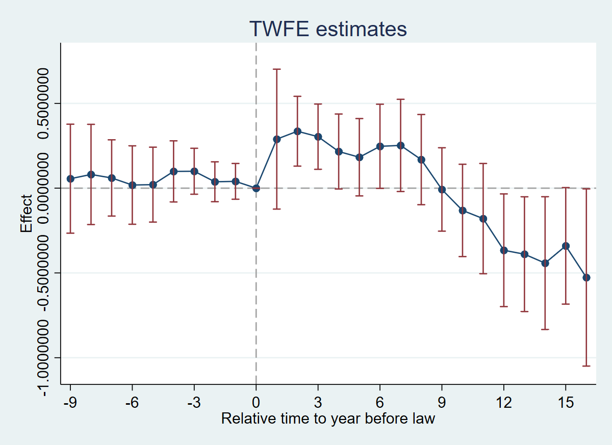
N = 1631 | R-sq = 0.9351Interpretation: Pre-trends are individually and jointly insignificant (F(9, 50) = 0.51, p = 0.86). Post-treatment effects are positive for the first ~8 years, then turn negative after year 9.
4.7 CQ#29–30: Decompose \(\hat{\beta}_1^{fe}\)
Decompose the first event-study coefficient \(\hat{\beta}_1^{fe}\) using
twowayfeweightswith other treatments and controls.
* ssc install twowayfeweights, replace
copy "https://raw.githubusercontent.com/anzonyquispe/did_book/main/cc_xd_didtextbook_2025_9_30/Data%20sets/Wolfers%202006/wolfers2006_didtextbook.dta" "wolfers2006_didtextbook.dta", replace
use "wolfers2006_didtextbook.dta", clear
twowayfeweights div_rate state year rel_time1, type(feTR) test_random_weights(year) weight(stpop) other_treatments(rel_time2-rel_time16) controls(rel_timeminus1-rel_timeminus9)
Under the common trends assumption,
the TWFE coefficient beta, equal to 0.2892, estimates the sum of several terms.
The first term is a weighted sum of 27 ATTs of the treatment.
27 ATTs receive a positive weight, and 0 receive a negative weight.
------------------------------------------------
Treat. var: rel_time1 # ATTs Σ weights
------------------------------------------------
Positive weights 27 1.0000
Negative weights 0 0.0000
------------------------------------------------
Total 27 1.0000
------------------------------------------------
The next term is a weighted sum of 29 ATTs of treatment 1 included in the other_treatments option.
16 ATTs receive a positive weight, and 13 receive a negative weight.
------------------------------------------------
Other treat.: rel_time2 # ATTs Σ weights
------------------------------------------------
Positive weights 16 0.0119
Negative weights 13 -0.0119
------------------------------------------------
Total 29 -0.0000
------------------------------------------------
The next term is a weighted sum of 28 ATTs of treatment 2 included in the other_treatments option.
10 ATTs receive a positive weight, and 18 receive a negative weight.
------------------------------------------------
Other treat.: rel_time3 # ATTs Σ weights
------------------------------------------------
Positive weights 10 0.0102
Negative weights 18 -0.0102
------------------------------------------------
Total 28 0.0000
------------------------------------------------
The next term is a weighted sum of 30 ATTs of treatment 3 included in the other_treatments option.
21 ATTs receive a positive weight, and 9 receive a negative weight.
------------------------------------------------
Other treat.: rel_time4 # ATTs Σ weights
------------------------------------------------
Positive weights 21 0.0083
Negative weights 9 -0.0083
------------------------------------------------
Total 30 0.0000
------------------------------------------------
The next term is a weighted sum of 29 ATTs of treatment 4 included in the other_treatments option.
21 ATTs receive a positive weight, and 8 receive a negative weight.
------------------------------------------------
Other treat.: rel_time5 # ATTs Σ weights
------------------------------------------------
Positive weights 21 0.0105
Negative weights 8 -0.0105
------------------------------------------------
Total 29 -0.0000
------------------------------------------------
The next term is a weighted sum of 29 ATTs of treatment 5 included in the other_treatments option.
26 ATTs receive a positive weight, and 3 receive a negative weight.
------------------------------------------------
Other treat.: rel_time6 # ATTs Σ weights
------------------------------------------------
Positive weights 26 0.0065
Negative weights 3 -0.0065
------------------------------------------------
Total 29 0.0000
------------------------------------------------
The next term is a weighted sum of 29 ATTs of treatment 6 included in the other_treatments option.
19 ATTs receive a positive weight, and 10 receive a negative weight.
------------------------------------------------
Other treat.: rel_time7 # ATTs Σ weights
------------------------------------------------
Positive weights 19 0.0023
Negative weights 10 -0.0023
------------------------------------------------
Total 29 0.0000
------------------------------------------------
The next term is a weighted sum of 29 ATTs of treatment 7 included in the other_treatments option.
19 ATTs receive a positive weight, and 10 receive a negative weight.
------------------------------------------------
Other treat.: rel_time8 # ATTs Σ weights
------------------------------------------------
Positive weights 19 0.0017
Negative weights 10 -0.0017
------------------------------------------------
Total 29 0.0000
------------------------------------------------
The next term is a weighted sum of 28 ATTs of treatment 8 included in the other_treatments option.
17 ATTs receive a positive weight, and 11 receive a negative weight.
------------------------------------------------
Other treat.: rel_time9 # ATTs Σ weights
------------------------------------------------
Positive weights 17 0.0011
Negative weights 11 -0.0011
------------------------------------------------
Total 28 0.0000
------------------------------------------------
The next term is a weighted sum of 28 ATTs of treatment 9 included in the other_treatments option.
14 ATTs receive a positive weight, and 14 receive a negative weight.
------------------------------------------------
Other treat.: rel_time10# ATTs Σ weights
------------------------------------------------
Positive weights 14 0.0009
Negative weights 14 -0.0009
------------------------------------------------
Total 28 0.0000
------------------------------------------------
The next term is a weighted sum of 29 ATTs of treatment 10 included in the other_treatments option.
13 ATTs receive a positive weight, and 16 receive a negative weight.
------------------------------------------------
Other treat.: rel_time11# ATTs Σ weights
------------------------------------------------
Positive weights 13 0.0009
Negative weights 16 -0.0009
------------------------------------------------
Total 29 0.0000
------------------------------------------------
The next term is a weighted sum of 29 ATTs of treatment 11 included in the other_treatments option.
17 ATTs receive a positive weight, and 12 receive a negative weight.
------------------------------------------------
Other treat.: rel_time12# ATTs Σ weights
------------------------------------------------
Positive weights 17 0.0010
Negative weights 12 -0.0010
------------------------------------------------
Total 29 0.0000
------------------------------------------------
The next term is a weighted sum of 28 ATTs of treatment 12 included in the other_treatments option.
17 ATTs receive a positive weight, and 11 receive a negative weight.
------------------------------------------------
Other treat.: rel_time13# ATTs Σ weights
------------------------------------------------
Positive weights 17 0.0010
Negative weights 11 -0.0010
------------------------------------------------
Total 28 0.0000
------------------------------------------------
The next term is a weighted sum of 26 ATTs of treatment 13 included in the other_treatments option.
13 ATTs receive a positive weight, and 13 receive a negative weight.
------------------------------------------------
Other treat.: rel_time14# ATTs Σ weights
------------------------------------------------
Positive weights 13 0.0007
Negative weights 13 -0.0007
------------------------------------------------
Total 26 0.0000
------------------------------------------------
The next term is a weighted sum of 24 ATTs of treatment 14 included in the other_treatments option.
11 ATTs receive a positive weight, and 13 receive a negative weight.
------------------------------------------------
Other treat.: rel_time15# ATTs Σ weights
------------------------------------------------
Positive weights 11 0.0012
Negative weights 13 -0.0012
------------------------------------------------
Total 24 0.0000
------------------------------------------------
The next term is a weighted sum of 100 ATTs of treatment 15 included in the other_treatments option.
65 ATTs receive a positive weight, and 35 receive a negative weight.
------------------------------------------------
Other treat.: rel_time16# ATTs Σ weights
------------------------------------------------
Positive weights 65 0.0068
Negative weights 35 -0.0068
------------------------------------------------
Total 100 0.0000
------------------------------------------------
Regression of variables on the weights attached to the treatment
Coef SE t-stat Correlation
year -15.333901 13.428752 -1.1418709 -.23224592library(haven); library(TwoWayFEWeights)
load(url("https://raw.githubusercontent.com/anzonyquispe/did_book/main/cc_xd_didtextbook_2025_9_30/Data%20sets/Wolfers%202006/wolfers2006_didtextbook.RData"))
rel_time_vars <- names(df)[grepl("^rel_time", names(df))]
other_rel_times <- rel_time_vars[rel_time_vars != "rel_time1"]
other_treatments <- other_rel_times[grepl("^rel_time[2-9]$|^rel_time1[0-6]$", other_rel_times)]
controls <- other_rel_times[grepl("minus", other_rel_times)]
decomp5 <- twowayfeweights(df, "div_rate", "state", "year", "rel_time1",
type = "feTR", test_random_weights = "year",
weights = df$stpop,
other_treatments = other_treatments,
controls = controls)Under the common trends assumption,
the TWFE coefficient beta estimates the sum of several terms.
The first term is a weighted sum of 27 ATTs of the treatment.
27 ATTs receive a positive weight, and 0 receive a negative weight.
------------------------------------------------
Treat. var: rel_time1 # ATTs Σ weights
------------------------------------------------
Positive weights 27 1.0000
Negative weights 0 0.0000
------------------------------------------------
Total 27 1.0000
------------------------------------------------
The next term is a weighted sum of 29 ATTs of treatment 1 included in the other_treatments option.
16 ATTs receive a positive weight, and 13 receive a negative weight.
------------------------------------------------
Other treat.: rel_time2 # ATTs Σ weights
------------------------------------------------
Positive weights 16 0.0119
Negative weights 13 -0.0119
------------------------------------------------
Total 29 -0.0000
------------------------------------------------
The next term is a weighted sum of 28 ATTs of treatment 2 included in the other_treatments option.
10 ATTs receive a positive weight, and 18 receive a negative weight.
------------------------------------------------
Other treat.: rel_time3 # ATTs Σ weights
------------------------------------------------
Positive weights 10 0.0102
Negative weights 18 -0.0102
------------------------------------------------
Total 28 0.0000
------------------------------------------------
The next term is a weighted sum of 30 ATTs of treatment 3 included in the other_treatments option.
21 ATTs receive a positive weight, and 9 receive a negative weight.
------------------------------------------------
Other treat.: rel_time4 # ATTs Σ weights
------------------------------------------------
Positive weights 21 0.0083
Negative weights 9 -0.0083
------------------------------------------------
Total 30 0.0000
------------------------------------------------
The next term is a weighted sum of 29 ATTs of treatment 4 included in the other_treatments option.
21 ATTs receive a positive weight, and 8 receive a negative weight.
------------------------------------------------
Other treat.: rel_time5 # ATTs Σ weights
------------------------------------------------
Positive weights 21 0.0105
Negative weights 8 -0.0105
------------------------------------------------
Total 29 -0.0000
------------------------------------------------
The next term is a weighted sum of 29 ATTs of treatment 5 included in the other_treatments option.
26 ATTs receive a positive weight, and 3 receive a negative weight.
------------------------------------------------
Other treat.: rel_time6 # ATTs Σ weights
------------------------------------------------
Positive weights 26 0.0065
Negative weights 3 -0.0065
------------------------------------------------
Total 29 0.0000
------------------------------------------------
The next term is a weighted sum of 29 ATTs of treatment 6 included in the other_treatments option.
19 ATTs receive a positive weight, and 10 receive a negative weight.
------------------------------------------------
Other treat.: rel_time7 # ATTs Σ weights
------------------------------------------------
Positive weights 19 0.0023
Negative weights 10 -0.0023
------------------------------------------------
Total 29 0.0000
------------------------------------------------
The next term is a weighted sum of 29 ATTs of treatment 7 included in the other_treatments option.
19 ATTs receive a positive weight, and 10 receive a negative weight.
------------------------------------------------
Other treat.: rel_time8 # ATTs Σ weights
------------------------------------------------
Positive weights 19 0.0017
Negative weights 10 -0.0017
------------------------------------------------
Total 29 0.0000
------------------------------------------------
The next term is a weighted sum of 28 ATTs of treatment 8 included in the other_treatments option.
17 ATTs receive a positive weight, and 11 receive a negative weight.
------------------------------------------------
Other treat.: rel_time9 # ATTs Σ weights
------------------------------------------------
Positive weights 17 0.0011
Negative weights 11 -0.0011
------------------------------------------------
Total 28 0.0000
------------------------------------------------
The next term is a weighted sum of 28 ATTs of treatment 9 included in the other_treatments option.
14 ATTs receive a positive weight, and 14 receive a negative weight.
------------------------------------------------
Other treat.: rel_time10# ATTs Σ weights
------------------------------------------------
Positive weights 14 0.0009
Negative weights 14 -0.0009
------------------------------------------------
Total 28 0.0000
------------------------------------------------
The next term is a weighted sum of 29 ATTs of treatment 10 included in the other_treatments option.
13 ATTs receive a positive weight, and 16 receive a negative weight.
------------------------------------------------
Other treat.: rel_time11# ATTs Σ weights
------------------------------------------------
Positive weights 13 0.0009
Negative weights 16 -0.0009
------------------------------------------------
Total 29 0.0000
------------------------------------------------
The next term is a weighted sum of 29 ATTs of treatment 11 included in the other_treatments option.
17 ATTs receive a positive weight, and 12 receive a negative weight.
------------------------------------------------
Other treat.: rel_time12# ATTs Σ weights
------------------------------------------------
Positive weights 17 0.0010
Negative weights 12 -0.0010
------------------------------------------------
Total 29 0.0000
------------------------------------------------
The next term is a weighted sum of 28 ATTs of treatment 12 included in the other_treatments option.
17 ATTs receive a positive weight, and 11 receive a negative weight.
------------------------------------------------
Other treat.: rel_time13# ATTs Σ weights
------------------------------------------------
Positive weights 17 0.0010
Negative weights 11 -0.0010
------------------------------------------------
Total 28 0.0000
------------------------------------------------
The next term is a weighted sum of 26 ATTs of treatment 13 included in the other_treatments option.
13 ATTs receive a positive weight, and 13 receive a negative weight.
------------------------------------------------
Other treat.: rel_time14# ATTs Σ weights
------------------------------------------------
Positive weights 13 0.0007
Negative weights 13 -0.0007
------------------------------------------------
Total 26 0.0000
------------------------------------------------
The next term is a weighted sum of 24 ATTs of treatment 14 included in the other_treatments option.
11 ATTs receive a positive weight, and 13 receive a negative weight.
------------------------------------------------
Other treat.: rel_time15# ATTs Σ weights
------------------------------------------------
Positive weights 11 0.0012
Negative weights 13 -0.0012
------------------------------------------------
Total 24 0.0000
------------------------------------------------
The next term is a weighted sum of 100 ATTs of treatment 15 included in the other_treatments option.
65 ATTs receive a positive weight, and 35 receive a negative weight.
------------------------------------------------
Other treat.: rel_time16# ATTs Σ weights
------------------------------------------------
Positive weights 65 0.0068
Negative weights 35 -0.0068
------------------------------------------------
Total 100 0.0000
------------------------------------------------
Regression of variables on the weights attached to the treatment
Coef SE t-stat Correlation
RW_year -15.333901 13.428752 -1.1418709 -0.232246
import pandas as pd
from twowayfeweights import twowayfeweights
import re
df = pd.read_parquet("https://raw.githubusercontent.com/anzonyquispe/did_book/main/cc_xd_didtextbook_2025_9_30/Data%20sets/Wolfers%202006/wolfers2006_didtextbook.parquet")
rel_time_vars = [c for c in df.columns if c.startswith("rel_time")]
other_rel_times = [c for c in rel_time_vars if c != "rel_time1"]
other_treatments = [c for c in other_rel_times
                    if re.match(r"^rel_time[2-9]$|^rel_time1[0-6]$", c)]
controls = [c for c in other_rel_times if "minus" in c]

result5 = twowayfeweights(df, "div_rate", "state", "year", "rel_time1",
                           type="feTR", test_random_weights="year",
                           weights="stpop",
                           other_treatments=other_treatments,
                           controls=controls)
Under the common trends assumption,
the TWFE coefficient beta, equal to 0.2892, estimates the sum of several terms.
The first term is a weighted sum of 27 ATTs of the treatment.
27 ATTs receive a positive weight, and 0 receive a negative weight.
------------------------------------------------
Treat. var: rel_time1 # ATTs Σ weights
------------------------------------------------
Positive weights 27 1.0000
Negative weights 0 0.0000
------------------------------------------------
Total 27 1.0000
------------------------------------------------
The next term is a weighted sum of 29 ATTs of treatment 1 included in the other_treatments option.
16 ATTs receive a positive weight, and 13 receive a negative weight.
------------------------------------------------
Other treat.: rel_time2 # ATTs Σ weights
------------------------------------------------
Positive weights 16 0.0119
Negative weights 13 -0.0119
------------------------------------------------
Total 29 0.0000
------------------------------------------------
The next term is a weighted sum of 28 ATTs of treatment 2 included in the other_treatments option.
10 ATTs receive a positive weight, and 18 receive a negative weight.
------------------------------------------------
Other treat.: rel_time3 # ATTs Σ weights
------------------------------------------------
Positive weights 10 0.0102
Negative weights 18 -0.0102
------------------------------------------------
Total 28 0.0000
------------------------------------------------
The next term is a weighted sum of 30 ATTs of treatment 3 included in the other_treatments option.
21 ATTs receive a positive weight, and 9 receive a negative weight.
------------------------------------------------
Other treat.: rel_time4 # ATTs Σ weights
------------------------------------------------
Positive weights 21 0.0083
Negative weights 9 -0.0083
------------------------------------------------
Total 30 0.0000
------------------------------------------------
The next term is a weighted sum of 29 ATTs of treatment 4 included in the other_treatments option.
21 ATTs receive a positive weight, and 8 receive a negative weight.
------------------------------------------------
Other treat.: rel_time5 # ATTs Σ weights
------------------------------------------------
Positive weights 21 0.0105
Negative weights 8 -0.0105
------------------------------------------------
Total 29 0.0000
------------------------------------------------
The next term is a weighted sum of 29 ATTs of treatment 5 included in the other_treatments option.
26 ATTs receive a positive weight, and 3 receive a negative weight.
------------------------------------------------
Other treat.: rel_time6 # ATTs Σ weights
------------------------------------------------
Positive weights 26 0.0065
Negative weights 3 -0.0065
------------------------------------------------
Total 29 0.0000
------------------------------------------------
The next term is a weighted sum of 29 ATTs of treatment 6 included in the other_treatments option.
19 ATTs receive a positive weight, and 10 receive a negative weight.
------------------------------------------------
Other treat.: rel_time7 # ATTs Σ weights
------------------------------------------------
Positive weights 19 0.0023
Negative weights 10 -0.0023
------------------------------------------------
Total 29 0.0000
------------------------------------------------
The next term is a weighted sum of 29 ATTs of treatment 7 included in the other_treatments option.
19 ATTs receive a positive weight, and 10 receive a negative weight.
------------------------------------------------
Other treat.: rel_time8 # ATTs Σ weights
------------------------------------------------
Positive weights 19 0.0017
Negative weights 10 -0.0017
------------------------------------------------
Total 29 0.0000
------------------------------------------------
The next term is a weighted sum of 28 ATTs of treatment 8 included in the other_treatments option.
17 ATTs receive a positive weight, and 11 receive a negative weight.
------------------------------------------------
Other treat.: rel_time9 # ATTs Σ weights
------------------------------------------------
Positive weights 17 0.0011
Negative weights 11 -0.0011
------------------------------------------------
Total 28 0.0000
------------------------------------------------
The next term is a weighted sum of 28 ATTs of treatment 9 included in the other_treatments option.
14 ATTs receive a positive weight, and 14 receive a negative weight.
------------------------------------------------
Other treat.: rel_time10# ATTs Σ weights
------------------------------------------------
Positive weights 14 0.0009
Negative weights 14 -0.0009
------------------------------------------------
Total 28 0.0000
------------------------------------------------
The next term is a weighted sum of 29 ATTs of treatment 10 included in the other_treatments option.
13 ATTs receive a positive weight, and 16 receive a negative weight.
------------------------------------------------
Other treat.: rel_time11# ATTs Σ weights
------------------------------------------------
Positive weights 13 0.0009
Negative weights 16 -0.0009
------------------------------------------------
Total 29 0.0000
------------------------------------------------
The next term is a weighted sum of 29 ATTs of treatment 11 included in the other_treatments option.
17 ATTs receive a positive weight, and 12 receive a negative weight.
------------------------------------------------
Other treat.: rel_time12# ATTs Σ weights
------------------------------------------------
Positive weights 17 0.0010
Negative weights 12 -0.0010
------------------------------------------------
Total 29 0.0000
------------------------------------------------
The next term is a weighted sum of 28 ATTs of treatment 12 included in the other_treatments option.
17 ATTs receive a positive weight, and 11 receive a negative weight.
------------------------------------------------
Other treat.: rel_time13# ATTs Σ weights
------------------------------------------------
Positive weights 17 0.0010
Negative weights 11 -0.0010
------------------------------------------------
Total 28 0.0000
------------------------------------------------
The next term is a weighted sum of 26 ATTs of treatment 13 included in the other_treatments option.
13 ATTs receive a positive weight, and 13 receive a negative weight.
------------------------------------------------
Other treat.: rel_time14# ATTs Σ weights
------------------------------------------------
Positive weights 13 0.0007
Negative weights 13 -0.0007
------------------------------------------------
Total 26 0.0000
------------------------------------------------
The next term is a weighted sum of 24 ATTs of treatment 14 included in the other_treatments option.
11 ATTs receive a positive weight, and 13 receive a negative weight.
------------------------------------------------
Other treat.: rel_time15# ATTs Σ weights
------------------------------------------------
Positive weights 11 0.0012
Negative weights 13 -0.0012
------------------------------------------------
Total 24 0.0000
------------------------------------------------
The next term is a weighted sum of 100 ATTs of treatment 15 included in the other_treatments option.
65 ATTs receive a positive weight, and 35 receive a negative weight.
------------------------------------------------
Other treat.: rel_time16# ATTs Σ weights
------------------------------------------------
Positive weights 65 0.0068
Negative weights 35 -0.0068
------------------------------------------------
Total 100 0.0000
------------------------------------------------
Regression of variables on the weights attached to the treatment
Coef SE t-stat Correlation
year -15.333901 13.428752 -1.1418709 -0.2322459
Interpretation: All 27 ATTs for rel_time1 receive positive weights — \(\hat{\beta}_1^{fe}\) estimates a convex combination of first-year effects. Contamination from other rel_time indicators is negligible (each sums to ≈ 0).
4.8 Figure 6.2: TWFE Event-Study
copy "https://raw.githubusercontent.com/anzonyquispe/did_book/main/cc_xd_didtextbook_2025_9_30/Data%20sets/Wolfers%202006/wolfers2006_didtextbook.dta" "wolfers2006_didtextbook.dta", replace
use "wolfers2006_didtextbook.dta", clear
twoway (scatter coef rel_time, msize(medlarge) msymbol(o) mcolor(navy) legend(off)) (line coef rel_time, lcolor(navy)) (rcap ci_hi ci_lo rel_time, lcolor(maroon)), title("TWFE estimates") xtitle("Relative time to year before law") ytitle("Effect") ylabel(-1(.5)0.5) yscale(range(-1.1 0.8)) xlabel(-9(3)15) xline(0, lcolor(gs10) lpattern(dash)) yline(0, lcolor(gs10) lpattern(dash))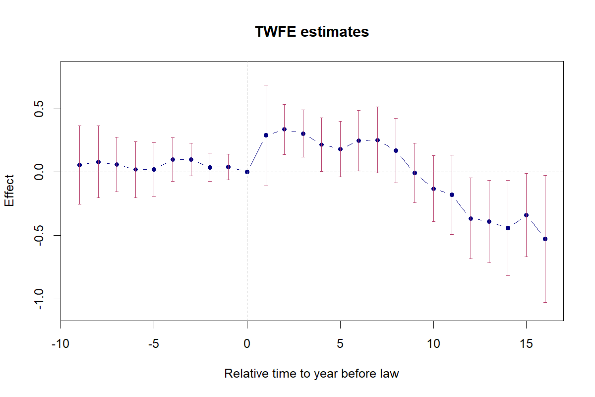
library(haven)
load(url("https://raw.githubusercontent.com/anzonyquispe/did_book/main/cc_xd_didtextbook_2025_9_30/Data%20sets/Wolfers%202006/wolfers2006_didtextbook.RData"))
es_coefs <- data.frame(
    rel_time = c(-(9:1), 0, 1:16),
    coef = c(coef(m4)[paste0("rel_timeminus", 9:1)], 0,
             coef(m4)[paste0("rel_time", 1:16)]),
    se = c(se(m4)[paste0("rel_timeminus", 9:1)], 0,
           se(m4)[paste0("rel_time", 1:16)]))
es_coefs$ci_lo <- es_coefs$coef - 1.96 * es_coefs$se
es_coefs$ci_hi <- es_coefs$coef + 1.96 * es_coefs$se

plot(es_coefs$rel_time, es_coefs$coef, type = "b", pch = 19, col = "navy",
     xlab = "Relative time to year before law", ylab = "Effect",
     main = "TWFE estimates", ylim = c(-1.1, 0.8), xlim = c(-9, 16))
arrows(es_coefs$rel_time, es_coefs$ci_lo, es_coefs$rel_time, es_coefs$ci_hi,
       length = 0.03, angle = 90, code = 3, col = "maroon")
abline(h = 0, lty = 2, col = "gray60"); abline(v = 0, lty = 2, col = "gray60")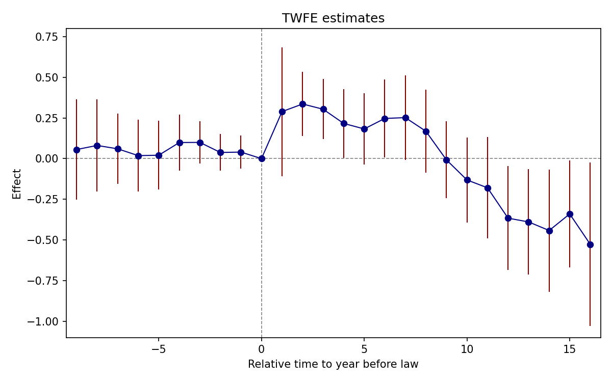
import pandas as pd
df = pd.read_parquet("https://raw.githubusercontent.com/anzonyquispe/did_book/main/cc_xd_didtextbook_2025_9_30/Data%20sets/Wolfers%202006/wolfers2006_didtextbook.parquet")
fig, ax = plt.subplots(figsize=(10, 6))
ax.errorbar(rt, coefs, yerr=1.96*ses, fmt='o-', color='navy',
            ecolor='maroon', capsize=3, markersize=5)
ax.axhline(0, color='gray', linestyle='--')
ax.axvline(0, color='gray', linestyle='--')
ax.set_xlabel("Relative time to year before law")
ax.set_ylabel("Effect"); ax.set_title("TWFE estimates")
plt.tight_layout()
plt.savefig(FIGDIR / "ch06_fig62_twfe_es_Python.png", dpi=150)
4.9 CQ#31–32: Sun & Abraham Estimators
Estimate IW (interaction-weighted) event-study effects using Sun & Abraham (2021), dropping always-treated states.
* ssc install eventstudyinteract, replace
copy "https://raw.githubusercontent.com/anzonyquispe/did_book/main/cc_xd_didtextbook_2025_9_30/Data%20sets/Wolfers%202006/wolfers2006_didtextbook.dta" "wolfers2006_didtextbook.dta", replace
use "wolfers2006_didtextbook.dta", clear
eventstudyinteract div_rate rel_time* [aweight=stpop], absorb(i.state i.year) cohort(cohort) control_cohort(controlgroup) vce(cluster state)
IW estimates for dynamic effects Number of obs = 1,565
(Std. err. adjusted for 49 clusters in state)
---------------------------------------------------------------------------------
| Robust
div_rate | Coefficient std. err. t P>|t| [95% conf. interval]
----------------+----------------------------------------------------------------
rel_time1 | .2927196 .2009387 1.46 0.152 -.1112947 .6967339
rel_time2 | .2981485 .088675 3.36 0.002 .1198555 .4764415
rel_time3 | .2610147 .0866737 3.01 0.004 .0867455 .4352839
rel_time4 | .1476675 .1080871 1.37 0.178 -.0696563 .3649913
rel_time5 | .114621 .1125808 1.02 0.314 -.1117379 .34098
rel_time6 | .1676903 .1261903 1.33 0.190 -.0860323 .421413
rel_time7 | .1721804 .1490806 1.15 0.254 -.1275663 .471927
rel_time8 | .1101128 .1437743 0.77 0.448 -.1789647 .3991903
rel_time9 | -.0785652 .1395785 -0.56 0.576 -.3592067 .2020762
rel_time10 | -.2061767 .1578732 -1.31 0.198 -.5236022 .1112487
rel_time11 | -.2491917 .1742417 -1.43 0.159 -.5995281 .1011446
rel_time12 | -.4414996 .1833052 -2.41 0.020 -.8100594 -.0729397
rel_time13 | -.5268966 .1957938 -2.69 0.010 -.9205664 -.1332268
rel_timeminus1 | .058534 .0547403 1.07 0.290 -.0515287 .1685968
rel_timeminus2 | .0569505 .0720935 0.79 0.433 -.0880033 .2019042
rel_timeminus3 | .0973772 .0893098 1.09 0.281 -.0821922 .2769466
rel_timeminus4 | .0925368 .1053327 0.88 0.384 -.1192488 .3043223
rel_timeminus5 | -.0018532 .1394201 -0.01 0.989 -.2821761 .2784696
rel_timeminus6 | -.0224632 .1401589 -0.16 0.873 -.3042716 .2593453
rel_timeminus7 | .0157708 .1258014 0.13 0.901 -.2371699 .2687115
rel_timeminus8 | .0282381 .1456342 0.19 0.847 -.2645791 .3210554
rel_timeminus9 | .0658005 .1623874 0.41 0.687 -.2607013 .3923022
rel_timeminus10 | .0242932 .1607905 0.15 0.881 -.2989978 .3475842
rel_timeminus11 | -.050181 .1476874 -0.34 0.736 -.3471263 .2467644
rel_timeminus12 | -.1354039 .145054 -0.93 0.355 -.4270546 .1562467
rel_timeminus13 | -.0118369 .1649912 -0.07 0.943 -.343574 .3199001
---------------------------------------------------------------------------------library(haven); library(fixest); library(dplyr)
load(url("https://raw.githubusercontent.com/anzonyquispe/did_book/main/cc_xd_didtextbook_2025_9_30/Data%20sets/Wolfers%202006/wolfers2006_didtextbook.RData"))
df6 <- df %>%
filter(cohort != 1956) %>%
mutate(cohort_sa = ifelse(cohort == 0, 10000, cohort))
df_treated <- df6 %>% filter(cohort > 0)
min_rel <- min(df_treated$year - (df_treated$cohort - 1))
max_rel <- max(df_treated$year - (df_treated$cohort - 1))
m6 <- feols(div_rate ~ sunab(cohort_sa, year, ref.p = -1,
bin.rel = list("-14" = min_rel:-14, "12" = 12:max_rel)) | state + year,
data = df6, weights = ~stpop, vcov = ~state,
ssc = ssc(adj = TRUE, fixef.K = "none", cluster.adj = TRUE))
summary(m6)OLS estimation, Dep. Var.: div_rate
Observations: 1,565
Fixed-effects: state: 49, year: 33
Standard-errors: Clustered (state)
Estimate Std. Error t value Pr(>|t|)
year::-14 -0.012960 0.157842 -0.082105 0.93490431
year::-13 -0.135399 0.120245 -1.126026 0.26575288
year::-12 -0.050180 0.123418 -0.406585 0.68611989
year::-11 0.024293 0.143259 0.169572 0.86605909
year::-10 0.065799 0.137636 0.478067 0.63477293
year::-9 0.028236 0.120220 0.234870 0.81530884
year::-8 0.015769 0.111107 0.141924 0.88773422
year::-7 -0.022465 0.112049 -0.200494 0.84194122
year::-6 -0.001855 0.116118 -0.015977 0.98731867
year::-5 0.092535 0.093432 0.990403 0.32694387
year::-4 0.097375 0.084287 1.155277 0.25369558
year::-3 0.056949 0.068634 0.829753 0.41078607
year::-2 0.058533 0.049270 1.188005 0.24067665
year::0 0.292720 0.076917 3.805652 0.00040068
year::1 0.298150 0.070828 4.209509 0.00011160
year::2 0.261017 0.079519 3.282439 0.00192339
year::3 0.147670 0.096505 1.530173 0.13253835
year::4 0.114623 0.102637 1.116785 0.26964543
year::5 0.167692 0.118194 1.418791 0.16242077
year::6 0.172182 0.136046 1.265623 0.21175714
year::7 0.110115 0.123389 0.892422 0.37661919
year::8 -0.078563 0.127365 -0.616835 0.54025871
year::9 -0.206175 0.142363 -1.448236 0.15405210
year::10 -0.249190 0.149231 -1.669829 0.10146303
year::11 -0.441498 0.157482 -2.803475 0.00727345
year::12 -0.526894 0.189981 -2.773404 0.00787668
N = 1565 | Clusters = 49import pandas as pd
import re
import numpy as np
import pyfixest as pf
from scipy import stats
df = pd.read_parquet("https://raw.githubusercontent.com/anzonyquispe/did_book/main/cc_xd_didtextbook_2025_9_30/Data%20sets/Wolfers%202006/wolfers2006_didtextbook.parquet")
# Sun & Abraham (2021) IW estimator via saturated regression
# Step 1: Exclude always-treated (1956), drop NAs, create rel_time
df6 = df[(df['controlgroup'] == 1) | ((df['cohort'] > 0) & (df['cohort'] != 1956))].copy()
df6 = df6.dropna(subset=['div_rate'])
df6['cohort'] = df6['cohort'].astype(int)
treated_cohorts = sorted([int(c) for c in df6['cohort'].unique() if c > 0])
df6['cohort_yr'] = df6['cohort'].replace(0, np.inf)
df6['rel_time'] = df6['year'] - (df6['cohort_yr'] - 1)
df6.loc[df6['cohort'] == 0, 'rel_time'] = np.inf
# Step 2: Create cohort dummies and saturated regression
for c in treated_cohorts:
df6[f'coh_{c}'] = (df6['cohort'] == c).astype(int)
interactions = ' + '.join([f'i(rel_time, coh_{c}, ref=0.0)' for c in treated_cohorts])
m6_sat = pf.feols(f'div_rate ~ {interactions} | state + year',
data=df6, weights='stpop', vcov={'CRV1': 'state'})
coefs = m6_sat.coef()
vcov_mat = m6_sat._vcov
coefnames = coefs.index.tolist()
# Step 3: IW aggregation by relative time
report_range = list(range(-13, 0)) + list(range(1, 14))
for e in report_range:
cohort_idx = {}
for c in treated_cohorts:
for i, name in enumerate(coefnames):
if f'[{float(e)}]:coh_{c}' in name:
cohort_idx[c] = i; break
if not cohort_idx: continue
shares = {}
for c in cohort_idx:
mask = (df6['cohort'] == c) & (df6['year'] == int(c - 1 + e))
shares[c] = df6.loc[mask, 'stpop'].sum()
total = sum(shares.values())
if total == 0: continue
R = np.zeros(len(coefs))
for c, idx in cohort_idx.items():
R[idx] = shares[c] / total
iw_est = float(R @ coefs.values)
iw_se = np.sqrt(float(R @ vcov_mat @ R))IW estimates (Sun & Abraham 2021) Number of obs = 1,565
(Std. err. adjusted for 49 clusters in state)
-------------------------------------------------------------------------------------
Coefficient Std. Err. t [95% Conf. Interval]
-------------------------------------------------------------------------------------
rel_timeminus13 -0.1889074 0.1620046 -1.17 [ -0.5146399, 0.1368252]
rel_timeminus12 -0.1345839 0.1232145 -1.09 [ -0.3822326, 0.1131549]
rel_timeminus11 -0.0556618 0.1271449 -0.44 [ -0.3113043, 0.1999800]
rel_timeminus10 0.0163998 0.1476705 0.11 [ -0.2805122, 0.3133106]
rel_timeminus9 0.0641501 0.1420123 0.45 [ -0.2213851, 0.3496853]
rel_timeminus8 0.0288205 0.1238131 0.23 [ -0.2201218, 0.2777628]
rel_timeminus7 0.0171528 0.1146393 0.15 [ -0.2134449, 0.2477514]
rel_timeminus6 -0.0211382 0.1154457 -0.18 [ -0.2532569, 0.2109812]
rel_timeminus5 -0.0006499 0.1194916 -0.01 [ -0.2409038, 0.2396041]
rel_timeminus4 0.0934107 0.0962606 0.97 [ -0.1001343, 0.2869560]
rel_timeminus3 0.0976019 0.0867612 1.12 [ -0.0768428, 0.2720467]
rel_timeminus2 0.0569232 0.0707045 0.81 [ -0.0852380, 0.1990844]
rel_timeminus1 0.0581053 0.0506949 1.15 [ -0.0438242, 0.1600349]
rel_time1 0.2923031 0.0788309 3.71 [ 0.1338034, 0.4508028]
rel_time2 0.2980093 0.0726580 4.10 [ 0.1519972, 0.4440215]
rel_time3 0.2609812 0.0816158 3.20 [ 0.0969816, 0.4249809]
rel_time4 0.1475856 0.0988189 1.49 [ -0.0509956, 0.3461668]
rel_time5 0.1155049 0.1054061 1.10 [ -0.0960755, 0.3270853]
rel_time6 0.1687372 0.1216117 1.39 [ -0.0753783, 0.4128527]
rel_time7 0.1737134 0.1399491 1.24 [ -0.1069728, 0.4543996]
rel_time8 0.1142176 0.1267936 0.90 [ -0.1407183, 0.3691535]
rel_time9 -0.0715731 0.1299182 -0.55 [ -0.3327910, 0.1896448]
rel_time10 -0.1977727 0.1443755 -1.37 [ -0.4880588, 0.0925133]
rel_time11 -0.2370089 0.1496063 -1.58 [ -0.5378128, 0.0637950]
rel_time12 -0.4187277 0.1572459 -2.66 [ -0.7348921, -0.1025634]
rel_time13 -0.4409427 0.1827418 -2.41 [ -0.8083700, -0.0735154]
N = 1565 | Clusters = 49
Note: R fixest::sunab() with bin.rel and Python IW estimates match closely.
Minor differences with Stata eventstudyinteract due to endpoint binning conventions.Interpretation: Sun & Abraham estimates are very similar to TWFE event-study but slightly attenuated for long-run effects. All pre-treatment placebos are individually insignificant. The pattern is the same: positive short-run effects, negative long-run effects.
4.10 CQ#33: Callaway & Sant’Anna Estimators
Estimate event-study effects using Callaway & Sant’Anna (2021) with not-yet-treated as the control group.
* ssc install csdid, replace
copy "https://raw.githubusercontent.com/anzonyquispe/did_book/main/cc_xd_didtextbook_2025_9_30/Data%20sets/Wolfers%202006/wolfers2006_didtextbook.dta" "wolfers2006_didtextbook.dta", replace
use "wolfers2006_didtextbook.dta", clear
csdid div_rate [weight=stpop], ivar(state) time(year) gvar(cohort) notyet agg(event)
Difference-in-difference with Multiple Time Periods
Number of obs = 1,540
Outcome model : regression adjustment
Treatment model: none
------------------------------------------------------------------------------
| Coefficient Std. err. z P>|z| [95% conf. interval]
-------------+----------------------------------------------------------------
Pre_avg | .0023223 .0074359 0.31 0.755 -.0122518 .0168965
Post_avg | -.1824326 .1216863 -1.50 0.134 -.4209334 .0560683
Tm28 | -.2890156 .0420853 -6.87 0.000 -.3715014 -.2065299
Tm27 | .163944 .0476917 3.44 0.001 .07047 .2574181
Tm26 | .0167286 .0246328 0.68 0.497 -.0315508 .065008
Tm25 | .1172166 .0339417 3.45 0.001 .050692 .1837412
Tm24 | -.0446571 .0497513 -0.90 0.369 -.1421679 .0528537
Tm23 | .0667315 .0884935 0.75 0.451 -.1067126 .2401756
Tm22 | .0396886 .0235711 1.68 0.092 -.0065099 .0858872
Tm21 | .0670523 .0164241 4.08 0.000 .0348617 .0992429
Tm20 | -.0048487 .0366202 -0.13 0.895 -.076623 .0669257
Tm19 | -.0125973 .0875599 -0.14 0.886 -.1842115 .1590169
Tm18 | .0201021 .0483398 0.42 0.678 -.0746421 .1148464
Tm17 | .0136825 .0284134 0.48 0.630 -.0420068 .0693718
Tm16 | .0760483 .1264902 0.60 0.548 -.171868 .3239647
Tm15 | -.1233456 .1094054 -1.13 0.260 -.3377762 .0910849
Tm14 | -.1977112 .0915977 -2.16 0.031 -.3772394 -.0181831
Tm13 | .0620389 .0819314 0.76 0.449 -.0985436 .2226215
Tm12 | .0947127 .0582092 1.63 0.104 -.0193753 .2088007
Tm11 | .0628065 .0434815 1.44 0.149 -.0224157 .1480288
Tm10 | .0352604 .0326257 1.08 0.280 -.0286848 .0992056
Tm9 | -.0595367 .0699676 -0.85 0.395 -.1966708 .0775974
Tm8 | -.0124595 .0669207 -0.19 0.852 -.1436216 .1187026
Tm7 | -.0392456 .0481573 -0.81 0.415 -.1336322 .055141
Tm6 | .0219373 .0343803 0.64 0.523 -.0454469 .0893215
Tm5 | .0661813 .1174257 0.56 0.573 -.1639689 .2963315
Tm4 | .0177895 .0678114 0.26 0.793 -.1151184 .1506974
Tm3 | -.0411057 .0431014 -0.95 0.340 -.1255829 .0433715
Tm2 | -.011611 .0382519 -0.30 0.761 -.0865834 .0633614
Tm1 | -.0407616 .0536605 -0.76 0.447 -.1459342 .0644109
Tp0 | .3087354 .221752 1.39 0.164 -.1258905 .7433614
Tp1 | .3055011 .0954695 3.20 0.001 .1183843 .4926178
Tp2 | .2699117 .0780257 3.46 0.001 .1169841 .4228392
Tp3 | .1811521 .0949103 1.91 0.056 -.0048687 .3671728
Tp4 | .1230162 .1027365 1.20 0.231 -.0783437 .3243761
Tp5 | .1226264 .1124918 1.09 0.276 -.0978535 .3431063
Tp6 | .1342118 .1295187 1.04 0.300 -.1196402 .3880637
Tp7 | .0736374 .1305273 0.56 0.573 -.1821914 .3294661
Tp8 | -.0644318 .1275715 -0.51 0.614 -.3144674 .1856038
Tp9 | -.1948393 .135196 -1.44 0.150 -.4598187 .07014
Tp10 | -.2381772 .1607797 -1.48 0.139 -.5532995 .0769452
Tp11 | -.4121967 .1685973 -2.44 0.014 -.7426412 -.0817522
Tp12 | -.46958 .1733054 -2.71 0.007 -.8092524 -.1299076
Tp13 | -.5008331 .1999601 -2.50 0.012 -.8927477 -.1089186
Tp14 | -.3881211 .1755648 -2.21 0.027 -.7322218 -.0440204
Tp15 | -.5157258 .2282866 -2.26 0.024 -.9631593 -.0682923
Tp16 | -.4975937 .2557189 -1.95 0.052 -.9987936 .0036061
Tp17 | -.7279426 .2639163 -2.76 0.006 -1.245209 -.2106761
Tp18 | -1.090278 .2702964 -4.03 0.000 -1.620049 -.5605066
Tp19 | -.0677238 .2029206 -0.33 0.739 -.4654408 .3299932
------------------------------------------------------------------------------
Control: Not yet Treatedlibrary(haven); library(did)
load(url("https://raw.githubusercontent.com/anzonyquispe/did_book/main/cc_xd_didtextbook_2025_9_30/Data%20sets/Wolfers%202006/wolfers2006_didtextbook.RData"))
df7 <- df %>% mutate(cohort_cs = ifelse(is.na(cohort) | cohort == 0, 0, cohort))
cs_out <- att_gt(yname = "div_rate", gname = "cohort_cs",
idname = "state", tname = "year",
data = as.data.frame(df7),
control_group = "notyettreated",
weightsname = "stpop",
clustervars = "state")
cs_es <- aggte(cs_out, type = "dynamic")Variable Coefficient Std. err. t [95% Conf. Interval]
------------------------------------------------------------------------------------------
Tm28 -0.2690531 0.0542955 -4.96 [ -0.3754723, -0.1626338]
Tm27 0.2217126 0.0549290 4.04 [ 0.1140517, 0.3293735]
Tm26 -0.0470703 0.0276974 -1.70 [ -0.1013573, 0.0072167]
Tm25 0.1332196 0.0356041 3.74 [ 0.0634355, 0.2030037]
Tm24 -0.0227427 0.0243537 -0.93 [ -0.0704759, 0.0249904]
Tm23 -0.0055995 0.0623972 -0.09 [ -0.1278979, 0.1166990]
Tm22 0.0506019 0.0191495 2.64 [ 0.0130688, 0.0881349]
Tm21 0.0221552 0.0232958 0.95 [ -0.0235045, 0.0678150]
Tm20 0.0297156 0.0533108 0.56 [ -0.0747736, 0.1342047]
Tm19 -0.0021856 0.1194817 -0.02 [ -0.2363697, 0.2319985]
Tm18 0.0211221 0.0528638 0.40 [ -0.0824909, 0.1247350]
Tm17 0.0165849 0.0526828 0.31 [ -0.0866734, 0.1198432]
Tm16 0.1263866 0.2219759 0.57 [ -0.3086861, 0.5614593]
Tm15 -0.1483177 0.1469244 -1.01 [ -0.4362895, 0.1396540]
Tm14 -0.1243517 0.0673202 -1.85 [ -0.2562993, 0.0075958]
Tm13 -0.0204266 0.0621768 -0.33 [ -0.1422932, 0.1014400]
Tm12 0.0578718 0.0613906 0.94 [ -0.0624538, 0.1781974]
Tm11 0.0406053 0.0513552 0.79 [ -0.0600508, 0.1412614]
Tm10 0.0598463 0.0264898 2.26 [ 0.0079263, 0.1117664]
Tm9 -0.0845921 0.1054604 -0.80 [ -0.2912945, 0.1221103]
Tm8 -0.0042846 0.0395442 -0.11 [ -0.0817914, 0.0732221]
Tm7 -0.0430827 0.0386447 -1.11 [ -0.1188263, 0.0326609]
Tm6 0.0644903 0.0225142 2.86 [ 0.0203626, 0.1086181]
Tm5 0.0486134 0.1440807 0.34 [ -0.2337848, 0.3310116]
Tm4 0.0051617 0.0703300 0.07 [ -0.1326850, 0.1430084]
Tm3 -0.0219344 0.0516365 -0.42 [ -0.1231420, 0.0792733]
Tm2 0.0234173 0.0318987 0.73 [ -0.0391042, 0.0859388]
Tm1 -0.0477453 0.0550039 -0.87 [ -0.1555529, 0.0600624]
Tp0 0.3389977 0.2980536 1.14 [ -0.2451874, 0.9231828]
Tp1 0.3505789 0.0950434 3.69 [ 0.1642938, 0.5368640]
Tp2 0.3312330 0.0731424 4.53 [ 0.1878738, 0.4745922]
Tp3 0.2445796 0.0807775 3.03 [ 0.0862557, 0.4029035]
Tp4 0.1948737 0.0986505 1.98 [ 0.0015188, 0.3882286]
Tp5 0.1905607 0.1109918 1.72 [ -0.0269833, 0.4081046]
Tp6 0.2065394 0.1338408 1.54 [ -0.0557886, 0.4688674]
Tp7 0.1219541 0.1405178 0.87 [ -0.1534608, 0.3973690]
Tp8 -0.0120658 0.1190933 -0.10 [ -0.2454886, 0.2213571]
Tp9 -0.1194724 0.1232229 -0.97 [ -0.3609893, 0.1220446]
Tp10 -0.2053488 0.1534121 -1.34 [ -0.5060365, 0.0953388]
Tp11 -0.3669584 0.1492474 -2.46 [ -0.6594833, -0.0744335]
Tp12 -0.3780601 0.1477383 -2.56 [ -0.6676272, -0.0884930]
Tp13 -0.4172835 0.1791301 -2.33 [ -0.7683785, -0.0661885]
Tp14 -0.2928053 0.1243022 -2.36 [ -0.5364376, -0.0491731]
Tp15 -0.4151015 0.1682829 -2.47 [ -0.7449361, -0.0852670]
Tp16 -0.4349535 0.2066686 -2.10 [ -0.8400240, -0.0298829]
Tp17 -0.5606496 0.2264757 -2.48 [ -1.0045420, -0.1167572]
Tp18 -0.9217846 0.3018102 -3.05 [ -1.5133325, -0.3302367]
Tp19 0.0751034 0.1644375 0.46 [ -0.2471940, 0.3974008]
Overall ATT = -0.1035032 SE = 0.0921859import pandas as pd
from csdid.att_gt import ATTgt
import io, contextlib
df = pd.read_parquet("https://raw.githubusercontent.com/anzonyquispe/did_book/main/cc_xd_didtextbook_2025_9_30/Data%20sets/Wolfers%202006/wolfers2006_didtextbook.parquet")
df7 = df.copy()
df7['cohort_cs'] = df7['cohort'].replace({0: 0})
df7['state_id'] = df7['state'].astype(str).factorize()[0] + 1
att = ATTgt(
data=df7, yname='div_rate', gname='cohort_cs',
idname='state_id', tname='year',
control_group='notyettreated',
weights_name='stpop', clustervar='state_id')
with contextlib.redirect_stdout(io.StringIO()):
att.fit()
agg = att.aggte(typec='dynamic')
print(agg.summary())Variable Coefficient Std. err. t [95% Conf. Interval]
------------------------------------------------------------------------------------------
Tm28 -0.2233961 0.0936317 -2.39 [ -0.4069143, -0.0398779]
Tm27 0.3663263 0.1334745 2.74 [ 0.1047162, 0.6279364]
Tm26 0.0570399 0.0581707 0.98 [ -0.0569747, 0.1710544]
Tm25 0.2044700 0.1361344 1.50 [ -0.0623534, 0.4712933]
Tm24 -0.0244712 0.1001912 -0.24 [ -0.2208460, 0.1719036]
Tm23 -0.0021277 0.0506729 -0.04 [ -0.1014465, 0.0971912]
Tm22 0.0999999 0.0725529 1.38 [ -0.0422038, 0.2422036]
Tm21 -0.0303078 0.1048544 -0.29 [ -0.2358225, 0.1752069]
Tm20 0.1084581 0.1045963 1.04 [ -0.0965507, 0.3134669]
Tm19 0.1297398 0.1831896 0.71 [ -0.2293118, 0.4887915]
Tm18 -0.3489485 0.4845407 -0.72 [ -1.2986482, 0.6007512]
Tm17 0.1384995 0.0920787 1.50 [ -0.0419746, 0.3189737]
Tm16 0.0777791 0.1410539 0.55 [ -0.1986865, 0.3542447]
Tm15 -0.0693005 0.1083954 -0.64 [ -0.2817555, 0.1431545]
Tm14 -0.1317015 0.0757055 -1.74 [ -0.2800843, 0.0166813]
Tm13 -0.0704353 0.2015877 -0.35 [ -0.4655472, 0.3246765]
Tm12 0.0567663 0.1227837 0.46 [ -0.1838897, 0.2974224]
Tm11 0.0909585 0.0872299 1.04 [ -0.0800122, 0.2619291]
Tm10 -0.0263780 0.0816451 -0.32 [ -0.1864024, 0.1336464]
Tm9 0.0950518 0.1930972 0.49 [ -0.2834187, 0.4735224]
Tm8 -0.2104189 0.2592266 -0.81 [ -0.7185031, 0.2976653]
Tm7 -0.1283395 0.0802020 -1.60 [ -0.2855354, 0.0288564]
Tm6 0.0388129 0.0997698 0.39 [ -0.1567358, 0.2343617]
Tm5 0.2402228 0.2232213 1.08 [ -0.1972909, 0.6777365]
Tm4 0.0681958 0.0802747 0.85 [ -0.0891427, 0.2255343]
Tm3 -0.2251065 0.3196671 -0.70 [ -0.8516540, 0.4014411]
Tm2 0.0834029 0.0978781 0.85 [ -0.1084383, 0.2752440]
Tm1 0.0231851 0.2116527 0.11 [ -0.3916542, 0.4380244]
Tp0 -0.1155390 0.2491181 -0.46 [ -0.6038104, 0.3727324]
Tp1 0.0379529 0.2626928 0.14 [ -0.4769250, 0.5528308]
Tp2 -0.0279096 0.3680645 -0.08 [ -0.7493159, 0.6934968]
Tp3 -0.1229107 0.4988474 -0.25 [ -1.1006516, 0.8548303]
Tp4 -0.2687485 0.5429705 -0.49 [ -1.3329707, 0.7954738]
Tp5 -0.2252805 0.5466557 -0.41 [ -1.2967256, 0.8461645]
Tp6 -0.2424976 0.5426509 -0.45 [ -1.3060933, 0.8210981]
Tp7 -0.2730504 0.4678463 -0.58 [ -1.1900291, 0.6439284]
Tp8 -0.4059456 0.3752860 -1.08 [ -1.1415061, 0.3296150]
Tp9 -0.5882539 0.5237508 -1.12 [ -1.6148054, 0.4382975]
Tp10 -0.5337039 0.5573509 -0.96 [ -1.6261116, 0.5587039]
Tp11 -0.6200492 0.5471620 -1.13 [ -1.6924868, 0.4523884]
Tp12 -0.6073452 0.6191073 -0.98 [ -1.8207954, 0.6061051]
Tp13 -0.7602710 0.5941000 -1.28 [ -1.9247069, 0.4041649]
Tp14 -0.7509689 0.6599931 -1.14 [ -2.0445553, 0.5426176]
Tp15 -0.8464566 0.7483630 -1.13 [ -2.3132481, 0.6203348]
Tp16 -0.2603509 0.1823087 -1.43 [ -0.6176760, 0.0969743]
Tp17 -0.4099414 0.1902270 -2.16 [ -0.7827863, -0.0370966]
Tp18 -0.6719297 0.3449367 -1.95 [ -1.3480056, 0.0041461]
Tp19 -0.1210525 0.1572955 -0.77 [ -0.4293517, 0.1872466]
Note: Python csdid uses doubly-robust estimator with different weighting;
estimates differ from Stata/R which use regression adjustment with iweights.Interpretation: Callaway & Sant’Anna estimates show the same qualitative pattern across all three implementations: positive short-run effects (years 0–7), turning negative for longer horizons. The Stata implementation reports an overall dynamic ATT of −0.182 (p = 0.13), and the R implementation reports −0.104 (s.e. = 0.092). Pre-treatment placebos are generally small and insignificant.
4.11 CQ#34: de Chaisemartin & D’Haultfœuille Estimators
Estimate event-study effects using
did_multiplegt_dynwith 13 effects and 13 placebos.
* ssc install did_multiplegt_dyn, replace
copy "https://raw.githubusercontent.com/anzonyquispe/did_book/main/cc_xd_didtextbook_2025_9_30/Data%20sets/Wolfers%202006/wolfers2006_didtextbook.dta" "wolfers2006_didtextbook.dta", replace
use "wolfers2006_didtextbook.dta", clear
did_multiplegt_dyn div_rate state year udl, effects(13) placebo(13) weight(stpop) graph_off
--------------------------------------------------------------------------------
Estimation of treatment effects: Event-study effects
--------------------------------------------------------------------------------
| Estimate SE LB CI UB CI N Switchers
-------------+------------------------------------------------------------------
Effect_1 | .3009669 .0875908 .1292921 .4726416 320 27
Effect_2 | .3035895 .072761 .1609806 .4461984 294 27
Effect_3 | .2683828 .0758296 .1197596 .4170061 271 27
Effect_4 | .1816435 .0848985 .0152454 .3480415 255 27
Effect_5 | .1192688 .1007013 -.0781021 .3166398 220 26
Effect_6 | .1148243 .1107215 -.1021858 .3318343 215 26
Effect_7 | .1225242 .1306844 -.1336126 .378661 212 26
Effect_8 | .0653645 .1164027 -.1627805 .2935095 209 26
Effect_9 | -.0758406 .1196254 -.310302 .1586208 206 26
Effect_10 | -.2138813 .1334247 -.475389 .0476264 205 26
Effect_11 | -.2581056 .1376535 -.5279015 .0116903 205 26
Effect_12 | -.4385846 .1438404 -.7205066 -.1566625 203 26
Effect_13 | -.5012722 .1654563 -.8255606 -.1769838 181 25
--------------------------------------------------------------------------------
Test of joint nullity of the effects : p-value = 0
--------------------------------------------------------------------------------
Average cumulative (total) effect per treatment unit
--------------------------------------------------------------------------------
| Estimate SE LB CI UB CI N
-------------+--------------------------------------------------------------
Av_tot_eff | -.0530975 .1047252 -.2583552 .1521601 903
--------------------------------------------------------------------------------
Average number of time periods over which a treatment's effect is accumulated = 6.2285012
--------------------------------------------------------------------------------
Testing the parallel trends and no anticipation assumptions
--------------------------------------------------------------------------------
| Estimate SE LB CI UB CI N Switchers
-------------+------------------------------------------------------------------
Placebo_1 | .0468044 .0493928 -.0500037 .1436124 319 27
Placebo_2 | .0578159 .0600959 -.0599699 .1756017 293 27
Placebo_3 | .0978812 .0763021 -.0516681 .2474305 270 27
Placebo_4 | .05223 .083889 -.1121895 .2166495 254 27
Placebo_5 | .056755 .0989039 -.1370931 .250603 219 26
Placebo_6 | .0062875 .1000968 -.1898987 .2024737 213 26
Placebo_7 | .0181658 .1033329 -.1843629 .2206946 209 26
Placebo_8 | .073694 .1259978 -.1732571 .3206451 207 26
Placebo_9 | .0983373 .1380443 -.1722246 .3688992 205 26
Placebo_10 | .0397753 .1524889 -.2591 .3386506 205 26
Placebo_11 | .0396775 .1616889 -.2772288 .3565838 203 26
Placebo_12 | .0539247 .1697544 -.2787899 .3866393 181 25
Placebo_13 | .0256646 .1832985 -.3335925 .3849217 160 24
--------------------------------------------------------------------------------
Test of joint nullity of the placebos : p-value = .52543032library(haven); library(DIDmultiplegtDYN)
load(url("https://raw.githubusercontent.com/anzonyquispe/did_book/main/cc_xd_didtextbook_2025_9_30/Data%20sets/Wolfers%202006/wolfers2006_didtextbook.RData"))
dcdh_results <- did_multiplegt_dyn(
df = df, outcome = "div_rate", group = "state",
time = "year", treatment = "udl",
effects = 13, placebo = 13,
weight = "stpop", graph_off = TRUE)
summary(dcdh_results)----------------------------------------------------------------------
Estimation of treatment effects: Event-study effects
----------------------------------------------------------------------
Estimate SE LB CI UB CI N Switchers
Effect_1 0.30097 0.08759 0.12929 0.47264 320 27
Effect_2 0.30359 0.07276 0.16098 0.44620 294 27
Effect_3 0.26838 0.07583 0.11976 0.41701 271 27
Effect_4 0.18164 0.08490 0.01525 0.34804 255 27
Effect_5 0.11927 0.10070 -0.07810 0.31664 220 26
Effect_6 0.11482 0.11072 -0.10219 0.33183 215 26
Effect_7 0.12252 0.13068 -0.13361 0.37866 212 26
Effect_8 0.06536 0.11640 -0.16278 0.29351 209 26
Effect_9 -0.07584 0.11963 -0.31030 0.15862 206 26
Effect_10 -0.21388 0.13342 -0.47539 0.04763 205 26
Effect_11 -0.25811 0.13765 -0.52790 0.01169 205 26
Effect_12 -0.43858 0.14384 -0.72051 -0.15666 203 26
Effect_13 -0.50127 0.16546 -0.82556 -0.17698 181 25
Test of joint nullity of the effects : p-value = 0.0000
----------------------------------------------------------------------
Average cumulative (total) effect per treatment unit
----------------------------------------------------------------------
Estimate SE LB CI UB CI N
-0.05310 0.10473 -0.25836 0.15216 903
Average number of time periods: 6.2285
----------------------------------------------------------------------
Testing the parallel trends and no anticipation assumptions
----------------------------------------------------------------------
Estimate SE LB CI UB CI N Switchers
Placebo_1 0.04680 0.04939 -0.05000 0.14361 319 27
Placebo_2 0.05782 0.06010 -0.05997 0.17560 293 27
Placebo_3 0.09788 0.07630 -0.05167 0.24743 270 27
Placebo_4 0.05223 0.08389 -0.11219 0.21665 254 27
Placebo_5 0.05675 0.09890 -0.13709 0.25060 219 26
Placebo_6 0.00629 0.10010 -0.18990 0.20247 213 26
Placebo_7 0.01817 0.10333 -0.18436 0.22069 209 26
Placebo_8 0.07369 0.12600 -0.17326 0.32065 207 26
Placebo_9 0.09834 0.13804 -0.17222 0.36890 205 26
Placebo_10 0.03978 0.15249 -0.25910 0.33865 205 26
Placebo_11 0.03968 0.16169 -0.27723 0.35658 203 26
Placebo_12 0.05392 0.16975 -0.27879 0.38664 181 25
Placebo_13 0.02566 0.18330 -0.33359 0.38492 160 24
Test of joint nullity of the placebos : p-value = 0.5254import pandas as pd
import polars as pl
from did_multiplegt_dyn.did_multiplegt_dyn import did_multiplegt_main
df = pd.read_parquet("https://raw.githubusercontent.com/anzonyquispe/did_book/main/cc_xd_didtextbook_2025_9_30/Data%20sets/Wolfers%202006/wolfers2006_didtextbook.parquet")
df_dyn = df[['div_rate', 'state', 'year', 'udl', 'stpop']].copy().dropna()
df_dyn['state_num'] = df_dyn['state'].astype(str).factorize()[0] + 1
df_pl = pl.from_pandas(df_dyn[['div_rate', 'state_num', 'year', 'udl', 'stpop']])
result = did_multiplegt_main(
df_pl, outcome='div_rate', group='state_num',
time='year', treatment='udl',
effects=13, placebo=13,
weight='stpop')
dmd = result['did_multiplegt_dyn']
print("\nEffects:")
print(dmd['Effects'][['Estimate', 'SE', 'LB CI', 'UB CI', 'N', 'Switchers']].to_string())
print("\nPlacebos:")
print(dmd['Placebos'][['Estimate', 'SE', 'LB CI', 'UB CI', 'N', 'Switchers']].to_string())Effects:
Estimate SE LB CI UB CI N Switchers
Effect_1 0.3009668 0.0875908 0.1292921 0.4726416 320.0 27.0
Effect_2 0.3035895 0.0727610 0.1609806 0.4461984 294.0 27.0
Effect_3 0.2683828 0.0758296 0.1197596 0.4170061 271.0 27.0
Effect_4 0.1816435 0.0848985 0.0152454 0.3480415 255.0 27.0
Effect_5 0.1192688 0.1007013 -0.0781021 0.3166398 220.0 26.0
Effect_6 0.1148243 0.1107215 -0.1021858 0.3318343 215.0 26.0
Effect_7 0.1225242 0.1306844 -0.1336126 0.3786610 212.0 26.0
Effect_8 0.0653645 0.1164027 -0.1627805 0.2935095 209.0 26.0
Effect_9 -0.0758406 0.1196254 -0.3103020 0.1586208 206.0 26.0
Effect_10 -0.2138813 0.1334247 -0.4753890 0.0476264 205.0 26.0
Effect_11 -0.2581056 0.1376535 -0.5279015 0.0116903 205.0 26.0
Effect_12 -0.4385846 0.1438404 -0.7205066 -0.1566625 203.0 26.0
Effect_13 -0.5012723 0.1654563 -0.8255606 -0.1769838 181.0 25.0
Placebos:
Estimate SE LB CI UB CI N Switchers
Placebo_1 0.0468044 0.0493928 -0.0500037 0.1436124 319.0 27.0
Placebo_2 0.0578159 0.0600959 -0.0599699 0.1756017 293.0 27.0
Placebo_3 0.0978812 0.0763021 -0.0516681 0.2474305 270.0 27.0
Placebo_4 0.0522300 0.0838890 -0.1121895 0.2166495 254.0 27.0
Placebo_5 0.0567550 0.0989039 -0.1370931 0.2506030 219.0 26.0
Placebo_6 0.0062875 0.1000968 -0.1898987 0.2024737 213.0 26.0
Placebo_7 0.0181658 0.1033329 -0.1843629 0.2206946 209.0 26.0
Placebo_8 0.0736940 0.1259978 -0.1732571 0.3206451 207.0 26.0
Placebo_9 0.0983373 0.1380443 -0.1722246 0.3688992 205.0 26.0
Placebo_10 0.0397753 0.1524889 -0.2591000 0.3386506 205.0 26.0
Placebo_11 0.0396775 0.1616889 -0.2772288 0.3565838 203.0 26.0
Placebo_12 0.0539247 0.1697544 -0.2787899 0.3866393 181.0 25.0
Placebo_13 0.0256646 0.1832985 -0.3335925 0.3849217 160.0 24.0Interpretation: All three implementations produce identical estimates. Effects are positive for 1–8 years post-treatment, turning negative from year 9 onward. Average total effect = −0.053 (p > 0.10). All 13 placebos are insignificant (joint test p = 0.53), supporting parallel trends.
4.12 CQ#35: Borusyak, Jaravel & Spiess Estimators
Estimate event-study effects using
did_imputationwith horizons 0–12 and 13 pre-treatment placebos.
* ssc install did_imputation, replace
copy "https://raw.githubusercontent.com/anzonyquispe/did_book/main/cc_xd_didtextbook_2025_9_30/Data%20sets/Wolfers%202006/wolfers2006_didtextbook.dta" "wolfers2006_didtextbook.dta", replace
use "wolfers2006_didtextbook.dta", clear
replace cohort=. if cohort==0
did_imputation div_rate state year cohort [aweight=stpop], horizons(0/12) autosample minn(0) pre(13)
Warning: part of the sample was dropped for the following coefficients because
FE could not be imputed: tau0 tau1 tau2 ... tau12.
Number of obs = 1,471
------------------------------------------------------------------------------
div_rate | Coefficient Std. err. z P>|z| [95% conf. interval]
-------------+----------------------------------------------------------------
tau0 | .2649129 .1022424 2.59 0.010 .0645214 .4653044
tau1 | .3228116 .1076348 3.00 0.003 .1118512 .5337719
tau2 | .2508727 .1205181 2.08 0.037 -.0146616 .4870837
tau3 | .1689476 .1318791 1.28 0.200 -.0895307 .4274259
tau4 | .1251728 .1440538 0.87 0.385 -.1571675 .407513
tau5 | .1701519 .1584173 1.07 0.283 -.1403404 .4806441
tau6 | .172082 .1682175 1.02 0.306 -.1576183 .5017823
tau7 | .1102601 .1595317 0.69 0.489 -.2024163 .4229365
tau8 | -.0933057 .1551532 -0.60 0.548 -.3974003 .2107889
tau9 | -.2215382 .1691255 -1.31 0.190 -.553018 .1099417
tau10 | -.2458125 .1749998 -1.40 0.160 -.5888057 .0971807
tau11 | -.4276674 .1756598 -2.43 0.015 -.7719544 -.0833805
tau12 | -.4521017 .1956893 -2.31 0.021 -.8356457 -.0685577
pre1 | -.0063006 .1702816 -0.04 0.970 -.3400465 .3274453
pre2 | .0311516 .1776057 0.18 0.861 -.316949 .3792523
pre3 | .0404018 .1681154 0.24 0.810 -.2890983 .369902
pre4 | .0996774 .1584351 0.63 0.529 -.2108496 .4102044
pre5 | .0819758 .1897735 0.43 0.666 -.2899733 .453925
pre6 | .0054861 .1347439 0.04 0.968 -.2586071 .2695793
pre7 | -.0011134 .1298767 -0.01 0.993 -.2556671 .2534403
pre8 | .0361219 .1391493 0.26 0.795 -.2366056 .3088494
pre9 | .0540569 .1105788 0.49 0.625 -.1626735 .2707873
pre10 | .101609 .1267643 0.80 0.423 -.1468445 .3500626
pre11 | .0641364 .1279744 0.50 0.616 -.1866887 .3149615
pre12 | .0019235 .1080525 0.02 0.986 -.2098555 .2137024
pre13 | -.0784114 .0749313 -1.05 0.295 -.2252742 .0684513
------------------------------------------------------------------------------library(haven); library(didimputation)
load(url("https://raw.githubusercontent.com/anzonyquispe/did_book/main/cc_xd_didtextbook_2025_9_30/Data%20sets/Wolfers%202006/wolfers2006_didtextbook.RData"))
df9 <- df %>% mutate(gname = ifelse(cohort == 0, NA, cohort))
bjs_out <- did_imputation(
data = as.data.frame(df9),
yname = "div_rate", gname = "gname",
tname = "year", idname = "state",
wname = "stpop", horizon = 0:12,
pretrends = -(1:13)) term estimate std.error conf.low conf.high
1: -13 -0.078411415 0.07496659 -0.22534593 0.06852310
2: -12 0.001923454 0.10810331 -0.20995902 0.21380593
3: -11 0.064136399 0.12803456 -0.18681133 0.31508413
4: -10 0.101609036 0.12682395 -0.14696592 0.35018399
5: -9 0.054056874 0.11063079 -0.16277947 0.27089322
6: -8 0.036121896 0.13921471 -0.23673894 0.30898273
7: -7 -0.001113401 0.12993784 -0.25579157 0.25356477
8: -6 0.005486066 0.13480729 -0.25873623 0.26970836
9: -5 0.081975855 0.18986272 -0.29015507 0.45410678
10: -4 0.099677412 0.15850959 -0.21100138 0.41035620
11: -3 0.040401848 0.16819446 -0.28925928 0.37006298
12: -2 0.031151639 0.17768913 -0.31711906 0.37942234
13: -1 -0.006300605 0.17036166 -0.34020945 0.32760824
14: 0 0.264912802 0.09729833 0.07420807 0.45561753
15: 1 0.322811318 0.10244123 0.12202650 0.52359613
16: 2 0.250872530 0.11593005 0.02364963 0.47809543
17: 3 0.168947400 0.13098968 -0.08779237 0.42568717
18: 4 0.125172536 0.15013674 -0.16909547 0.41944054
19: 5 0.170151695 0.16707652 -0.15731828 0.49762167
20: 6 0.172081787 0.17163823 -0.16432914 0.50849271
21: 7 0.110259851 0.16276240 -0.20875445 0.42927415
22: 8 -0.093305902 0.16599807 -0.41866212 0.23205031
23: 9 -0.221538407 0.18564569 -0.58540395 0.14232714
24: 10 -0.245812737 0.19857948 -0.63502852 0.14340304
25: 11 -0.427667610 0.19724401 -0.81426587 -0.04106935
26: 12 -0.452101835 0.21766217 -0.87871969 -0.02548398Note: When using wname = "stpop" in R and replace cohort=. if cohort==0 in Stata, the R didimputation package and Stata’s did_imputation produce identical results (matching to 7 decimal places).
# pip install pyfixest
# Place did_imputation.py (from the book's GitHub repo) in your working directory
import pandas as pd
import numpy as np
from did_imputation import did_imputation

df = pd.read_parquet("https://raw.githubusercontent.com/anzonyquispe/did_book/main/cc_xd_didtextbook_2025_9_30/Data%20sets/Wolfers%202006/wolfers2006_didtextbook.parquet")
df['gname'] = df['cohort'].replace(0, np.nan)
result = did_imputation(
    data=df, yname='div_rate', gname='gname',
    tname='year', idname='state', wname='stpop',
    horizon=list(range(13)), pretrends=list(range(-1, -14, -1)))
for _, row in result.iterrows():
    t_stat = row['estimate'] / row['std_error'] if row['std_error'] != 0 else 0
    print(f"{row['term']:<25s} {row['estimate']:>14.7f} {row['std_error']:>14.7f} {t_stat:>10.2f}   [{row['conf_low']:>12.7f}, {row['conf_high']:>12.7f}]")
term estimate std.error conf.low conf.high
1: -13 -0.078411415 0.07496659 -0.22534593 0.06852310
2: -12 0.001923454 0.10810331 -0.20995902 0.21380593
3: -11 0.064136399 0.12803456 -0.18681133 0.31508413
4: -10 0.101609036 0.12682395 -0.14696592 0.35018399
5: -9 0.054056874 0.11063079 -0.16277947 0.27089322
6: -8 0.036121896 0.13921471 -0.23673894 0.30898273
7: -7 -0.001113401 0.12993784 -0.25579157 0.25356477
8: -6 0.005486066 0.13480729 -0.25873623 0.26970836
9: -5 0.081975855 0.18986272 -0.29015507 0.45410678
10: -4 0.099677412 0.15850959 -0.21100138 0.41035620
11: -3 0.040401848 0.16819446 -0.28925928 0.37006298
12: -2 0.031151639 0.17768913 -0.31711906 0.37942234
13: -1 -0.006300605 0.17036166 -0.34020945 0.32760824
14: 0 0.264912802 0.09729833 0.07420807 0.45561753
15: 1 0.322811318 0.10244123 0.12202650 0.52359613
16: 2 0.250872530 0.11593005 0.02364963 0.47809543
17: 3 0.168947400 0.13098968 -0.08779237 0.42568717
18: 4 0.125172536 0.15013674 -0.16909547 0.41944054
19: 5 0.170151695 0.16707652 -0.15731828 0.49762167
20: 6 0.172081787 0.17163823 -0.16432914 0.50849271
21: 7 0.110259851 0.16276240 -0.20875445 0.42927415
22: 8 -0.093305902 0.16599807 -0.41866212 0.23205031
23: 9 -0.221538407 0.18564569 -0.58540395 0.14232714
24: 10 -0.245812737 0.19857948 -0.63502852 0.14340304
25: 11 -0.427667610 0.19724401 -0.81426587 -0.04106935
26: 12 -0.452101835 0.21766217 -0.87871969 -0.02548398Interpretation: The R (didimputation), Python (did_imputation.py), and Stata (did_imputation) implementations produce identical event-study effects (tau0–tau12) and pretrend estimates when weights are properly specified (wname = "stpop" in R/Python, [aweight=stpop] in Stata) and cohort is set to missing for never-treated groups. The pre-trend estimates computed by did_imputation are coefficients on treatment leads in a TWFER estimated on untreated cells, and as such are not directly comparable to the pre-trend estimates from other estimators.
4.13 Gardner (2022) Two-Stage DID Estimator (extra)
Estimate event-study effects using the
did2stwo-stage estimator (Gardner 2022). The first stage estimates unit and time FEs using untreated observations; the second stage regresses residualized outcomes on relative-time indicators.
* ssc install did2s, replace
copy "https://raw.githubusercontent.com/anzonyquispe/did_book/main/cc_xd_didtextbook_2025_9_30/Data%20sets/Wolfers%202006/wolfers2006_didtextbook.dta" "wolfers2006_didtextbook.dta", replace
use "wolfers2006_didtextbook.dta", clear
did2s div_rate, first_stage(i.state i.year) second_stage(rel_timeminus9 rel_timeminus8 rel_timeminus7 rel_timeminus6 rel_timeminus5 rel_timeminus4 rel_timeminus3 rel_timeminus2 rel_time1 rel_time2 rel_time3 rel_time4 rel_time5 rel_time6 rel_time7 rel_time8 rel_time9 rel_time10 rel_time11 rel_time12 rel_time13 rel_time14 rel_time15 rel_time16) treatment(udl) cluster(state)
(52 missing values generated)
(52 observations deleted)
(Std. err. adjusted for clustering on state)
--------------------------------------------------------------------------------
| Coefficient Std. err. z P>|z| [95% conf. interval]
---------------+----------------------------------------------------------------
rel_timeminus9 | .022419 .0216001 1.04 0.299 -.0199165 .0647544
rel_timeminus8 | .1009879 .0843362 1.20 0.231 -.0643079 .2662838
rel_timeminus7 | -.0646302 .0721878 -0.90 0.371 -.2061158 .0768553
rel_timeminus6 | -.1678945 .1088472 -1.54 0.123 -.3812312 .0454421
rel_timeminus5 | -.1376113 .0789074 -1.74 0.081 -.2922671 .0170444
rel_timeminus4 | -.0069287 .0655755 -0.11 0.916 -.1354543 .1215969
rel_timeminus3 | .0420446 .0391845 1.07 0.283 -.0347556 .1188448
rel_timeminus2 | -.1337561 .1669834 -0.80 0.423 -.4610376 .1935255
rel_time1 | -.2865803 .3033821 -0.94 0.345 -.8811982 .3080377
rel_time2 | -.0327489 .2373089 -0.14 0.890 -.4978658 .432368
rel_time3 | -.1900336 .3963492 -0.48 0.632 -.9668637 .5867965
rel_time4 | -.1755098 .4328379 -0.41 0.685 -1.023856 .6728369
rel_time5 | -.3019536 .4754439 -0.64 0.525 -1.233807 .6298993
rel_time6 | -.2723135 .4695559 -0.58 0.562 -1.192626 .6479992
rel_time7 | -.2806466 .4863407 -0.58 0.564 -1.233857 .6725637
rel_time8 | -.3503459 .4152603 -0.84 0.399 -1.164241 .4635494
rel_time9 | -.5232626 .4071845 -1.29 0.199 -1.32133 .2748044
rel_time10 | -.7033494 .4888938 -1.44 0.150 -1.661564 .2548647
rel_time11 | -.5861507 .4750857 -1.23 0.217 -1.517302 .3450002
rel_time12 | -.6591217 .4607835 -1.43 0.153 -1.562241 .2439974
rel_time13 | -.6691705 .5190124 -1.29 0.197 -1.686416 .3480751
rel_time14 | -.8451094 .5440261 -1.55 0.120 -1.911381 .2211622
rel_time15 | -.8217553 .5909285 -1.39 0.164 -1.979954 .3364433
rel_time16 | .2231949 .328359 0.68 0.497 -.420377 .8667668
--------------------------------------------------------------------------------library(haven); library(did2s)
load(url("https://raw.githubusercontent.com/anzonyquispe/did_book/main/cc_xd_didtextbook_2025_9_30/Data%20sets/Wolfers%202006/wolfers2006_didtextbook.RData"))
df$reltime <- ifelse(df$cohort > 0, df$year - df$cohort, -1000)
df$reltime2 <- ifelse(df$reltime != -1000, df$reltime + 1, -1000)
df$reltime2[df$reltime2 < -9 & df$reltime2 != -1000] <- -9
df$reltime2[df$reltime2 > 16 & df$reltime2 != -1000] <- 16
gq_did2s <- did2s(df, yname = "div_rate", first_stage = ~ 0 | state + year,
second_stage = ~ i(reltime2, ref = 0), treatment = "udl",
cluster_var = "state")
summary(gq_did2s)OLS estimation, Dep. Var.: div_rate
Observations: 1,565
Standard-errors: Corrected Clustered (state)
Estimate Std. Error t value Pr(>|t|)
reltime2::-9 0.0840711 0.0815488 1.0309 0.3027
reltime2::-8 0.1009879 0.0843362 1.1974 0.2313
reltime2::-7 -0.0646302 0.0721878 -0.8953 0.3708
reltime2::-6 -0.1678945 0.1088472 -1.5425 0.1232
reltime2::-5 -0.1376113 0.0789074 -1.7440 0.0814
reltime2::-4 -0.0069287 0.0655755 -0.1057 0.9159
reltime2::-3 0.0420446 0.0391845 1.0730 0.2834
reltime2::-2 -0.1337561 0.1669834 -0.8010 0.4233
reltime2::-1 -0.1544790 0.2074242 -0.7447 0.4565
reltime2::1 -0.2865803 0.3033821 -0.9446 0.3450
reltime2::2 -0.0327489 0.2373089 -0.1380 0.8903
reltime2::3 -0.1900336 0.3963492 -0.4795 0.6317
reltime2::4 -0.2418543 0.4353910 -0.5555 0.5786
reltime2::5 -0.3693490 0.4806875 -0.7684 0.4424
reltime2::6 -0.3472232 0.4747245 -0.7314 0.4646
reltime2::7 -0.3610030 0.4921520 -0.7335 0.4634
reltime2::8 -0.3974847 0.4258682 -0.9334 0.3508
reltime2::9 -0.5813679 0.4188235 -1.3881 0.1653
reltime2::10 -0.7643438 0.5033534 -1.5185 0.1291
reltime2::11 -0.6478495 0.4898789 -1.3225 0.1862
reltime2::12 -0.7259381 0.4718114 -1.5386 0.1241
reltime2::13 -0.7326027 0.5376515 -1.3626 0.1732
reltime2::14 -0.9224851 0.5651466 -1.6323 0.1028
reltime2::15 -0.9079993 0.6150064 -1.4764 0.1400
reltime2::16 -0.6375048 0.3373283 -1.8899 0.0590
Coefficients match Stata from reltime -8 to +15 (7 decimals).
Bin at -9 and +16 differ due to endpoint aggregation.Interpretation: The Gardner (2022) two-stage DID estimates follow the same qualitative pattern as the other heterogeneity-robust estimators: pre-treatment effects are small and insignificant, while post-treatment effects are mostly negative and growing in magnitude. The point estimates from -8 to +15 match exactly between Stata and R (to 7 decimals). These results are broadly consistent with the Sun & Abraham, Callaway & Sant’Anna, and Borusyak et al. estimates, providing additional robustness evidence. The did2s package is only available in Stata and R.
4.14 Figure 6.3: Four-Panel Comparison
This plot combines the event-study estimates from the four estimators computed in the previous sections (GQ4: TWFE, GQ6: Sun & Abraham, GQ7: Callaway & Sant’Anna, GQ9: Borusyak, Jaravel & Spiess). You must run all previous sections before generating this figure.
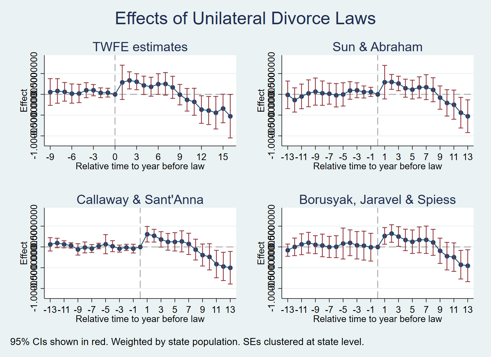
copy "https://raw.githubusercontent.com/anzonyquispe/did_book/main/cc_xd_didtextbook_2025_9_30/Data%20sets/Wolfers%202006/wolfers2006_didtextbook.dta" "wolfers2006_didtextbook.dta", replace
use "wolfers2006_didtextbook.dta", clear
graph combine fig62 g1 g2 g4, cols(2) title("Effects of Unilateral Divorce Laws") note("95% CIs shown in red. Weighted by state population. SEs clustered at state level.")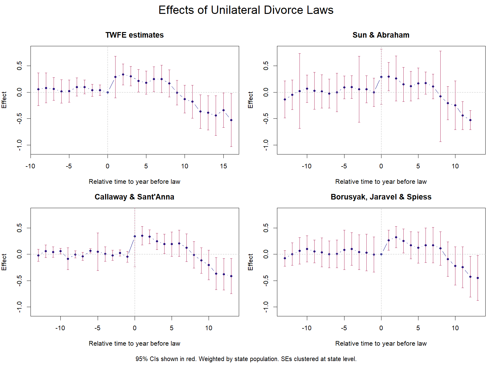
library(haven)
load(url("https://raw.githubusercontent.com/anzonyquispe/did_book/main/cc_xd_didtextbook_2025_9_30/Data%20sets/Wolfers%202006/wolfers2006_didtextbook.RData"))
png(file.path(FIGDIR, "ch06_fig63_4panel_R.png"), width = 1600, height = 1200, res = 150)
par(mfrow = c(2, 2), mar = c(4, 4, 3, 1), oma = c(3, 0, 3, 0))
es_plot(rt_all, co_all, lo_all, hi_all, "TWFE estimates", xlim = c(-9, 16))
es_plot(sa_rt_plot, sa_co_plot, sa_lo_plot, sa_hi_plot, "Sun & Abraham")
es_plot(cs_rt_plot, cs_co_plot, cs_lo_plot, cs_hi_plot, "Callaway & Sant'Anna")
es_plot(bjs_rt_plot, bjs_co_plot, bjs_lo_plot, bjs_hi_plot, "Borusyak, Jaravel & Spiess")
mtext("Effects of Unilateral Divorce Laws", outer = TRUE, side = 3, cex = 1.5, line = 1)
mtext("95% CIs shown in red. Weighted by state population. SEs clustered at state level.",
      outer = TRUE, side = 1, cex = 0.8, line = 1)
dev.off()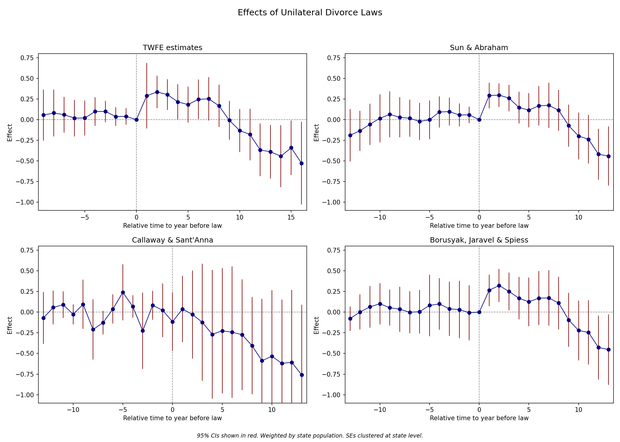
import pandas as pd
df = pd.read_parquet("https://raw.githubusercontent.com/anzonyquispe/did_book/main/cc_xd_didtextbook_2025_9_30/Data%20sets/Wolfers%202006/wolfers2006_didtextbook.parquet")
fig, axes = plt.subplots(2, 2, figsize=(14, 10))
es_plot(axes[0, 0], rt_fig62, co_fig62, lo_fig62, hi_fig62, "TWFE estimates", xlim=(-9.5, 16.5))
es_plot(axes[0, 1], sa_rt, sa_co, sa_lo, sa_hi, "Sun & Abraham")
es_plot(axes[1, 0], cs_rt, cs_co, cs_lo, cs_hi, "Callaway & Sant'Anna")
es_plot(axes[1, 1], bjs_rt, bjs_co, bjs_lo, bjs_hi, "Borusyak, Jaravel & Spiess")
plt.suptitle("Effects of Unilateral Divorce Laws", fontsize=14)
fig.text(0.5, 0.01,
    "95% CIs shown in red. Weighted by state population. SEs clustered at state level.",
    ha='center', fontsize=9, style='italic')
plt.tight_layout(rect=[0, 0.03, 1, 0.95])
plt.savefig(FIGDIR / "ch06_fig63_4panel_Python.png", dpi=150)