2  Synthetic Data Generation

3 Data Generation Process

We generate synthetic panel data following the simulation design in Callaway & Sant’Anna (2021), with heterogeneous treatment effects that vary by:

1. Treatment cohort (when units first receive treatment)
2. Time since treatment (dynamic effects)

This design creates a challenging test case where traditional TWFE would produce biased estimates.

3.1 Data Generating Process

The outcome variable follows:

\[Y_{it} = \alpha_i + \lambda_t + \tau_{g,t} \cdot D_{it} + \varepsilon_{it}\]

Where:

• \(\alpha_i\): Unit fixed effect
• \(\lambda_t\): Time fixed effect
• \(D_{it}\): Treatment indicator (1 if unit \(i\) is treated at time \(t\))
• \(\tau_{g,t}\): Treatment effect that varies by cohort \(g\) and calendar time \(t\)
• \(\varepsilon_{it} \sim N(0, 1)\): Idiosyncratic error

3.1.1 Heterogeneous Treatment Effects

We specify treatment effects that:

• Increase with time since treatment (dynamic effects)
• Vary by treatment cohort (cohort heterogeneity)

\[\tau_{g,t} = \tau_0 + \delta_g + \gamma \cdot (t - g)\]

Where:

• \(\tau_0 = 1.0\): Base treatment effect
• \(\delta_g\): Cohort-specific shift (earlier cohorts have larger effects)
• \(\gamma = 0.1\): Effect growth per period since treatment

3.2 R Implementation

set.seed(20240115)

# Parameters
n_units <- 10000
n_periods <- 10
base_year <- 2010
years <- base_year:(base_year + n_periods - 1)

# Treatment cohorts and probabilities
treat_cohorts <- c(0, 2012, 2014, 2016, 2018)  # 0 = never treated
cohort_probs <- c(0.30, 0.20, 0.20, 0.20, 0.10)

# Cohort-specific effect shifts (earlier cohorts have larger effects)
cohort_effects <- c(0, 0.5, 0.3, 0.1, 0.0)  # delta_g for each cohort
names(cohort_effects) <- treat_cohorts

# Base effect and dynamic effect parameter
tau_0 <- 1.0
gamma <- 0.1  # Effect growth per period

cat("Generating panel data...\n")

Generating panel data...

cat("Units:", format(n_units, big.mark = ","), "\n")

Units: 10,000 

cat("Periods:", n_periods, "\n")

Periods: 10 

cat("Total observations:", format(n_units * n_periods, big.mark = ","), "\n")

Total observations: 1e+05 

# Generate unit-level data
unit_data <- data.frame(
  id = 1:n_units,
  g = sample(treat_cohorts, n_units, replace = TRUE, prob = cohort_probs),
  unit_fe = rnorm(n_units, 0, 1)
)

# Time fixed effects
time_fe_vals <- seq(-0.2, 0.2, length.out = n_periods)
names(time_fe_vals) <- years

# Expand to panel
cat("Creating panel structure...\n")

Creating panel structure...

panel <- expand.grid(id = 1:n_units, year = years)
panel <- merge(panel, unit_data, by = "id")

# Add time fixed effects
panel$time_fe <- time_fe_vals[as.character(panel$year)]

# Treatment indicator
panel$treated <- (panel$g > 0) & (panel$year >= panel$g)

# Calculate heterogeneous treatment effects
# tau_gt = tau_0 + delta_g + gamma * (t - g) for treated observations
panel$tau_gt <- 0
treated_idx <- panel$treated
panel$tau_gt[treated_idx] <- tau_0 +
  cohort_effects[as.character(panel$g[treated_idx])] +
  gamma * (panel$year[treated_idx] - panel$g[treated_idx])

# Generate outcome
panel$y <- 2 + panel$unit_fe + panel$time_fe +
           panel$tau_gt * as.integer(panel$treated) +
           rnorm(nrow(panel), 0, 1)

# Rename for standard DiD notation
panel$first_treat <- panel$g

# Sort for efficiency
panel <- panel[order(panel$id, panel$year), ]

cat("\nData generation complete!\n")

Data generation complete!

cat("Treatment group distribution:\n")

Treatment group distribution:

print(table(unit_data$g))

   0 2012 2014 2016 2018 
2991 2018 1928 2046 1017 

# Save for use in subsequent chapters
saveRDS(panel, "sim_data.rds")
write.csv(panel[, c("id", "year", "y", "first_treat", "treated")],
          "sim_data.csv", row.names = FALSE)

3.3 True Treatment Effects

Let’s calculate and display the true treatment effects for validation:

library(dplyr)

Attaching package: 'dplyr'

The following objects are masked from 'package:stats':

    filter, lag

The following objects are masked from 'package:base':

    intersect, setdiff, setequal, union

# Calculate true ATT by cohort and event time
true_effects <- panel %>%
  filter(treated) %>%
  mutate(event_time = year - g) %>%
  group_by(g, event_time) %>%
  summarise(
    true_att = mean(tau_gt),
    n_obs = n(),
    .groups = "drop"
  )

# Overall ATT
overall_att <- mean(panel$tau_gt[panel$treated])
cat("Overall true ATT:", round(overall_att, 4), "\n\n")

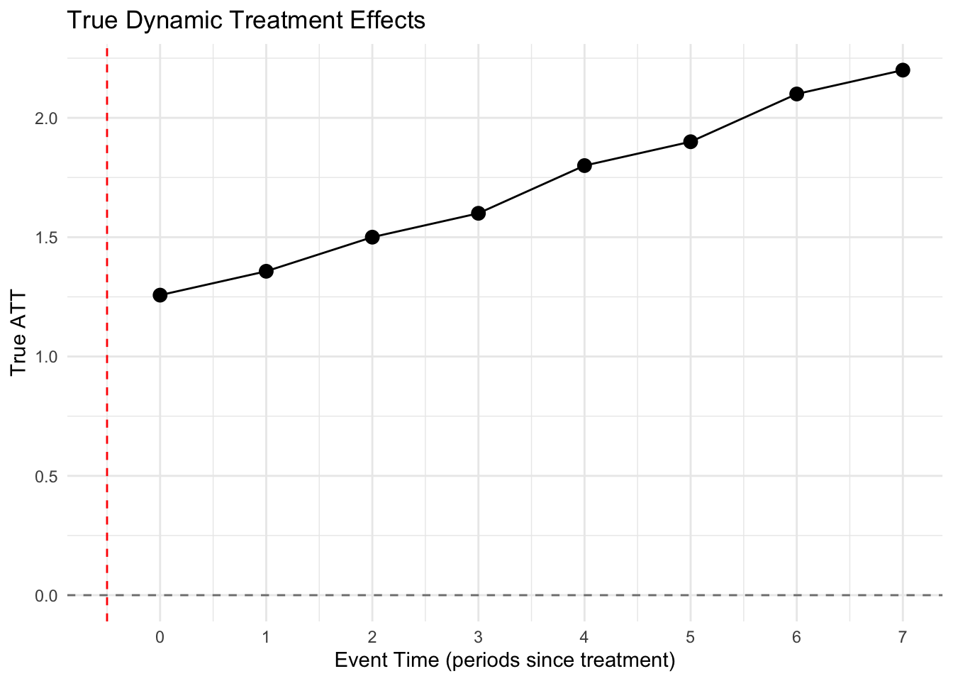
Overall true ATT: 1.5869 

# ATT by cohort
cat("True ATT by cohort:\n")

True ATT by cohort:

cohort_att <- true_effects %>%
  group_by(g) %>%
  summarise(true_att = mean(true_att), .groups = "drop")
print(cohort_att)

# A tibble: 4 × 2
      g true_att
  <dbl>    <dbl>
1  2012     1.85
2  2014     1.55
3  2016     1.25
4  2018     1.05

# Dynamic effects (event study)
cat("\nTrue dynamic effects (averaged across cohorts):\n")

True dynamic effects (averaged across cohorts):

dynamic_effects <- true_effects %>%
  group_by(event_time) %>%
  summarise(true_att = weighted.mean(true_att, n_obs), .groups = "drop")
print(dynamic_effects)

# A tibble: 8 × 2
  event_time true_att
       <dbl>    <dbl>
1          0     1.26
2          1     1.36
3          2     1.50
4          3     1.60
5          4     1.80
6          5     1.90
7          6     2.1 
8          7     2.2 

library(ggplot2)

ggplot(dynamic_effects, aes(x = event_time, y = true_att)) +
  geom_point(size = 3) +
  geom_line() +
  geom_hline(yintercept = 0, linetype = "dashed", color = "gray50") +
  geom_vline(xintercept = -0.5, linetype = "dashed", color = "red") +
  labs(
    x = "Event Time (periods since treatment)",
    y = "True ATT",
    title = "True Dynamic Treatment Effects"
  ) +
  theme_minimal() +
  scale_x_continuous(breaks = -7:7)

True treatment effects by event time

3.4 Python Implementation

For Python packages, we’ll load the same data:

import numpy as np
import pandas as pd

# Load the data generated by R for consistency
df = pd.read_csv("sim_data.csv")
print(f"Loaded {len(df):,} observations")
print(f"Units: {df['id'].nunique():,}")
print(f"Periods: {df['year'].nunique()}")
print(f"\nTreatment cohort distribution:")
print(df.groupby('first_treat')['id'].nunique())

3.5 Data Summary

cat("Final dataset dimensions:\n")

Final dataset dimensions:

cat("Rows:", format(nrow(panel), big.mark = ","), "\n")

Rows: 10,000,000 

cat("Columns:", ncol(panel), "\n")

Columns: 9 

cat("\nColumn names:", paste(names(panel), collapse = ", "), "\n")

Column names: id, year, g, unit_fe, time_fe, treated, tau_gt, y, first_treat 

cat("\nTreatment status:\n")

Treatment status:

cat("Treated observations:", format(sum(panel$treated), big.mark = ","), "\n")

Treated observations: 3,802,782 

cat("Control observations:", format(sum(!panel$treated), big.mark = ","), "\n")

Control observations: 6,197,218 

cat("\nMemory usage:", format(object.size(panel), units = "MB"), "\n")

Memory usage: 610.4 Mb