3  R Package Analysis

4 R Packages for Staggered DiD

This chapter benchmarks four major R packages for difference-in-differences with staggered treatment adoption.

# Load required packages
library(dplyr)
library(ggplot2)

# Load the simulated data
panel <- readRDS("sim_data.rds")

cat("Data loaded:\n")

Data loaded:

cat("Observations:", format(nrow(panel), big.mark = ","), "\n")

Observations: 10,000,000 

cat("Units:", format(length(unique(panel$id)), big.mark = ","), "\n")

Units: 1,000,000 

# Calculate true overall ATT for comparison
true_overall_att <- mean(panel$tau_gt[panel$treated])
cat("True overall ATT:", round(true_overall_att, 4), "\n")

True overall ATT: 1.5869 

# Initialize results storage
results <- list()

4.1 1. Callaway & Sant’Anna (did package)

The did package implements the method from Callaway & Sant’Anna (2021), estimating group-time average treatment effects and aggregating them.

Method: Doubly-robust estimation combining outcome regression and propensity score weighting.

library(did)

cat("Running did::att_gt()...\n")

Running did::att_gt()...

cat("This may take several minutes with 1M units.\n\n")

This may take several minutes with 1M units.

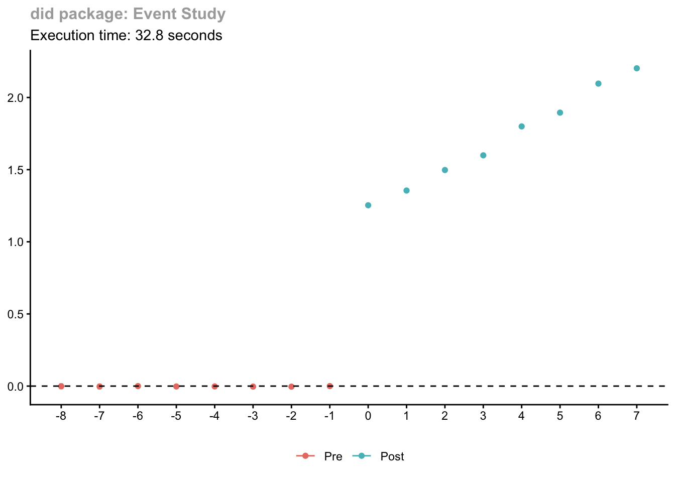
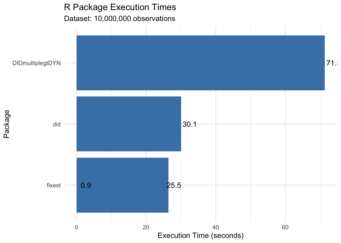
# Time the estimation
start_time <- Sys.time()

# Estimate group-time ATTs
# Using subset for large data (full data may require significant memory)
out_cs <- att_gt(
  yname = "y",
  gname = "first_treat",
  idname = "id",
  tname = "year",
  data = panel,
  control_group = "nevertreated",
  est_method = "dr",  # doubly robust
  base_period = "universal"
)

cs_time <- as.numeric(difftime(Sys.time(), start_time, units = "secs"))

cat("\nExecution time:", round(cs_time, 2), "seconds\n")

Execution time: 31.49 seconds

# Aggregate to overall ATT
agg_cs <- aggte(out_cs, type = "simple")
cat("\nOverall ATT estimate:", round(agg_cs$overall.att, 4), "\n")

Overall ATT estimate: 1.5846 

cat("Standard error:", round(agg_cs$overall.se, 4), "\n")

Standard error: 0.0019 

cat("True ATT:", round(true_overall_att, 4), "\n")

True ATT: 1.5869 

# Event study aggregation
es_cs <- aggte(out_cs, type = "dynamic")

results$did <- list(
  package = "did",
  method = "Callaway & Sant'Anna",
  time = cs_time,
  att = agg_cs$overall.att,
  se = agg_cs$overall.se,
  event_study = es_cs
)

# Plot event study
ggdid(es_cs) +
  labs(title = "did package: Event Study",
       subtitle = paste("Execution time:", round(cs_time, 1), "seconds"))

Event study: Callaway & Sant’Anna (did package)

4.2 2. de Chaisemartin & D’Haultfoeuille (DIDmultiplegtDYN)

The DIDmultiplegtDYN package implements the method from de Chaisemartin & D’Haultfoeuille, robust to heterogeneous treatment effects.

Method: Comparing switchers to non-switchers at each period.

# Check if package is available
if (requireNamespace("DIDmultiplegtDYN", quietly = TRUE)) {
  library(DIDmultiplegtDYN)
  library(dplyr)  # for pipe operator

  cat("Running DIDmultiplegtDYN::did_multiplegt_dyn()...\n")
  cat("This estimator can be slow with large datasets.\n\n")

  # Prepare data - DIDmultiplegtDYN needs treatment as binary
  panel_dcdh <- panel %>%
    mutate(D = as.integer(treated)) %>%
    select(id, year, y, D)

  start_time <- Sys.time()

  # Note: For very large datasets, this may require sampling
  # The package is computationally intensive
  tryCatch({
    out_dcdh <- did_multiplegt_dyn(
      df = panel_dcdh,
      outcome = "y",
      group = "id",
      time = "year",
      treatment = "D",
      effects = 5,  # Number of event-study effects
      placebo = 3,  # Number of pre-treatment placebos
      cluster = "id",
      graph_off = TRUE
    )

    dcdh_time <- as.numeric(difftime(Sys.time(), start_time, units = "secs"))

    cat("\nExecution time:", round(dcdh_time, 2), "seconds\n")
    print(summary(out_dcdh))

    # Extract ATT from results$ATE
    dcdh_att <- out_dcdh$results$ATE

    cat("\nAverage Total Effect (ATT):", round(dcdh_att, 4), "\n")
    cat("True ATT:", round(true_overall_att, 4), "\n")

    results$didmultiplegt <- list(
      package = "DIDmultiplegtDYN",
      method = "de Chaisemartin & D'Haultfoeuille",
      time = dcdh_time,
      att = dcdh_att,
      output = out_dcdh
    )
  }, error = function(e) {
    cat("Error running DIDmultiplegtDYN:", e$message, "\n")
    cat("This package may have memory constraints with 1M observations.\n")
    cat("Consider using a subsample for this estimator.\n")

    results$didmultiplegt <<- list(
      package = "DIDmultiplegtDYN",
      method = "de Chaisemartin & D'Haultfoeuille",
      time = NA,
      error = e$message
    )
  })

} else {
  cat("Package DIDmultiplegtDYN not installed.\n")
  cat("Install with: install.packages('DIDmultiplegtDYN')\n")

  results$didmultiplegt <- list(
    package = "DIDmultiplegtDYN",
    method = "de Chaisemartin & D'Haultfoeuille",
    time = NA,
    error = "Package not installed"
  )
}

Running DIDmultiplegtDYN::did_multiplegt_dyn()...
This estimator can be slow with large datasets.

Error running DIDmultiplegtDYN: vector memory limit of 36.0 Gb reached, see mem.maxVSize() 
This package may have memory constraints with 1M observations.
Consider using a subsample for this estimator.

4.2.1 Alternative: Using a subsample

Due to computational constraints, we may need to use a subsample:

if (requireNamespace("DIDmultiplegtDYN", quietly = TRUE) &&
    (is.null(results$didmultiplegt$time) || is.na(results$didmultiplegt$time))) {

  library(DIDmultiplegtDYN)
  library(dplyr)  # for pipe operator

  cat("Running DIDmultiplegtDYN on 10% subsample...\n")

  # Sample 10% of units
  set.seed(123)
  sample_ids <- sample(unique(panel$id), size = 100000)
  panel_sample <- panel %>%
    filter(id %in% sample_ids) %>%
    mutate(D = as.integer(treated)) %>%
    select(id, year, y, D)

  cat("Subsample size:", format(nrow(panel_sample), big.mark = ","), "\n\n")

  start_time <- Sys.time()

  tryCatch({
    out_dcdh_sample <- did_multiplegt_dyn(
      df = panel_sample,
      outcome = "y",
      group = "id",
      time = "year",
      treatment = "D",
      effects = 5,
      placebo = 3,
      cluster = "id",
      graph_off = TRUE
    )

    dcdh_time_sample <- as.numeric(difftime(Sys.time(), start_time, units = "secs"))

    cat("\nExecution time (10% sample):", round(dcdh_time_sample, 2), "seconds\n")
    cat("Estimated full data time:", round(dcdh_time_sample * 10, 2), "seconds\n")
    print(summary(out_dcdh_sample))

    # Extract ATT from results$ATE
    dcdh_att_sample <- out_dcdh_sample$results$ATE

    cat("\nAverage Total Effect (ATT):", round(dcdh_att_sample, 4), "\n")
    cat("True ATT:", round(true_overall_att, 4), "\n")

    results$didmultiplegt_sample <- list(
      package = "DIDmultiplegtDYN",
      method = "de Chaisemartin & D'Haultfoeuille (10% sample)",
      time = dcdh_time_sample,
      att = dcdh_att_sample,
      estimated_full_time = dcdh_time_sample * 10,
      output = out_dcdh_sample
    )
  }, error = function(e) {
    cat("Error:", e$message, "\n")
  })
}

Running DIDmultiplegtDYN on 10% subsample...
Subsample size: 1,000,000 


Execution time (10% sample): 76.09 seconds
Estimated full data time: 760.9 seconds

----------------------------------------------------------------------
       Estimation of treatment effects: Event-study effects
----------------------------------------------------------------------
             Estimate SE      LB CI   UB CI   N       Switchers
Effect_1     1.23956  0.00624 1.22734 1.25179 279,385 70,318   
Effect_2     1.35506  0.00621 1.34288 1.36723 279,385 70,318   
Effect_3     1.49808  0.00708 1.48420 1.51196 189,344 60,368   
Effect_4     1.59630  0.00709 1.58241 1.61020 189,344 60,368   
Effect_5     1.79333  0.00890 1.77589 1.81077 109,652 40,338   

Test of joint nullity of the effects : p-value = 0.0000
----------------------------------------------------------------------
    Average cumulative (total) effect per treatment unit
----------------------------------------------------------------------
 Estimate        SE     LB CI     UB CI         N Switchers 
  1.46362   0.00528   1.45327   1.47398   719,844   301,710 
Average number of time periods over which a treatment effect is accumulated: 2.7683

----------------------------------------------------------------------
     Testing the parallel trends and no anticipation assumptions
----------------------------------------------------------------------
             Estimate SE      LB CI    UB CI    N       Switchers
Placebo_1    -0.00871 0.00624 -0.02094 0.00353  279,385 70,318   
Placebo_2    -0.01505 0.00749 -0.02974 -0.00037 179,385 50,409   
Placebo_3    -0.00406 0.00887 -0.02144 0.01333  109,773 40,459   

Test of joint nullity of the placebos : p-value = 0.2133


The development of this package was funded by the European Union.
ERC REALLYCREDIBLE - GA N. 101043899
NULL

Average Total Effect (ATT): 1.4636 0.0053 1.4533 1.474 719844 301710 719844 301710 
True ATT: 1.5869 

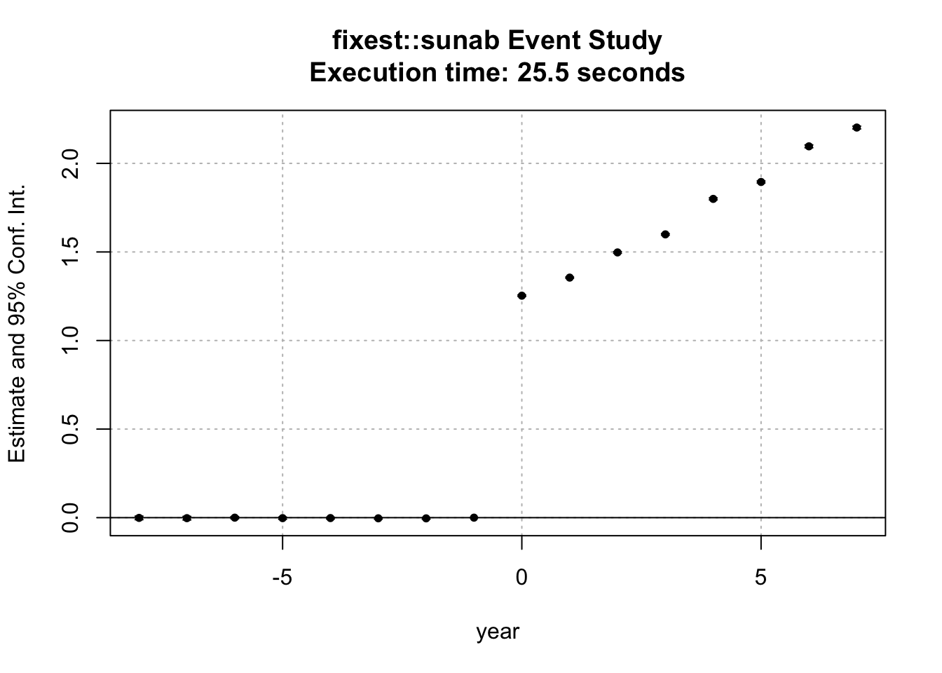
4.3 3. Sun & Abraham (fixest::sunab)

The fixest package provides the interaction-weighted estimator from Sun & Abraham (2021) through the sunab() function.

Method: Cohort-specific coefficients with clean controls.

library(fixest)

cat("Running fixest::feols() with sunab()...\n\n")

Running fixest::feols() with sunab()...

# Create cohort variable for sunab
panel_sa <- panel %>%
  mutate(
    cohort = ifelse(first_treat == 0, Inf, first_treat),  # Never-treated = Inf
    rel_time = ifelse(first_treat == 0, -1000, year - first_treat)  # Relative time
  )

start_time <- Sys.time()

# Sun & Abraham estimation using sunab
out_sa <- feols(
  y ~ sunab(cohort, year) | id + year,
  data = panel_sa,
  cluster = ~id
)

sa_time <- as.numeric(difftime(Sys.time(), start_time, units = "secs"))

cat("Execution time:", round(sa_time, 2), "seconds\n\n")

Execution time: 27.16 seconds

# Summary
summary(out_sa, agg = "ATT")

OLS estimation, Dep. Var.: y
Observations: 10,000,000
Fixed-effects: id: 1,000,000,  year: 10
Standard-errors: Clustered (id) 
    Estimate Std. Error t value  Pr(>|t|)    
ATT  1.58456   0.001775 892.853 < 2.2e-16 ***
---
Signif. codes:  0 '***' 0.001 '**' 0.01 '*' 0.05 '.' 0.1 ' ' 1
RMSE: 0.948956     Adj. R2: 0.636526
                 Within R2: 0.14887 

# Get aggregated ATT - fixest aggregate returns different structure
agg_sa <- summary(out_sa, agg = "ATT")

# Extract ATT from the aggregated coefficients
sa_coefs <- coef(agg_sa)
sa_ses <- se(agg_sa)

# Filter to post-treatment effects (event time >= 0) and compute mean
post_idx <- grep("^year::", names(sa_coefs))
if (length(post_idx) > 0) {
  # Get event times from coefficient names
  event_times <- as.numeric(gsub("year::", "", names(sa_coefs)[post_idx]))
  post_treatment <- event_times >= 0
  sa_att <- mean(sa_coefs[post_idx][post_treatment], na.rm = TRUE)
  sa_se <- mean(sa_ses[post_idx][post_treatment], na.rm = TRUE)
} else {
  sa_att <- mean(sa_coefs, na.rm = TRUE)
  sa_se <- mean(sa_ses, na.rm = TRUE)
}

cat("\nOverall ATT estimate (post-treatment avg):", round(sa_att, 4), "\n")

Overall ATT estimate (post-treatment avg): 1.5846 

cat("True ATT:", round(true_overall_att, 4), "\n")

True ATT: 1.5869 

results$sunab <- list(
  package = "fixest",
  method = "Sun & Abraham (sunab)",
  time = sa_time,
  att = sa_att,
  se = sa_se,
  model = out_sa
)

# Event study plot
iplot(out_sa,
      main = paste("fixest::sunab Event Study\nExecution time:",
                   round(sa_time, 1), "seconds"))

Event study: Sun & Abraham (fixest::sunab)

4.4 4. Imputation Estimator (didimputation)

The didimputation package implements the imputation approach from Borusyak, Jaravel & Spiess (2024).

Method: Impute counterfactual outcomes for treated units using never-treated/not-yet-treated.

if (requireNamespace("didimputation", quietly = TRUE)) {
  library(didimputation)

  cat("Running didimputation::did_imputation()...\n\n")

  # Prepare data
  panel_imp <- panel %>%
    mutate(
      first_treat = ifelse(first_treat == 0, NA_integer_, first_treat),
      rel_time = ifelse(is.na(first_treat), NA_integer_, year - first_treat)
    )

  start_time <- Sys.time()

  tryCatch({
    out_imp <- did_imputation(
      data = panel_imp,
      yname = "y",
      gname = "first_treat",
      tname = "year",
      idname = "id",
      first_stage = ~ 0 | id + year,
      horizon = TRUE,
      pretrends = TRUE
    )

    imp_time <- as.numeric(difftime(Sys.time(), start_time, units = "secs"))

    cat("Execution time:", round(imp_time, 2), "seconds\n\n")
    print(out_imp)

    # Extract overall ATT
    att_rows <- out_imp$term >= 0
    overall_att_imp <- mean(out_imp$estimate[att_rows])

    cat("\nOverall ATT (post-treatment avg):", round(overall_att_imp, 4), "\n")
    cat("True ATT:", round(true_overall_att, 4), "\n")

    results$didimputation <- list(
      package = "didimputation",
      method = "Borusyak, Jaravel & Spiess",
      time = imp_time,
      att = overall_att_imp,
      output = out_imp
    )
  }, error = function(e) {
    cat("Error running didimputation:", e$message, "\n")
    results$didimputation <<- list(
      package = "didimputation",
      method = "Borusyak, Jaravel & Spiess",
      time = NA,
      error = e$message
    )
  })

} else {
  cat("Package didimputation not installed.\n")
  cat("Install with: install.packages('didimputation')\n")

  results$didimputation <- list(
    package = "didimputation",
    method = "Borusyak, Jaravel & Spiess",
    time = NA,
    error = "Package not installed"
  )
}

Running didimputation::did_imputation()...

Error running didimputation: LU factorization of .gCMatrix failed: out of memory or near-singular 

if (!is.null(results$didimputation$output)) {
  out_imp <- results$didimputation$output
  imp_time <- results$didimputation$time

  ggplot(out_imp, aes(x = term, y = estimate)) +
    geom_point() +
    geom_errorbar(aes(ymin = conf.low, ymax = conf.high), width = 0.2) +
    geom_hline(yintercept = 0, linetype = "dashed") +
    geom_vline(xintercept = -0.5, linetype = "dashed", color = "red") +
    labs(
      x = "Event Time",
      y = "Estimate",
      title = "didimputation Event Study",
      subtitle = paste("Execution time:", round(imp_time, 1), "seconds")
    ) +
    theme_minimal()
}

4.5 5. Traditional TWFE (Biased Baseline)

For comparison, let’s also run traditional two-way fixed effects, which is known to be biased with heterogeneous effects:

library(fixest)

cat("Running traditional TWFE for comparison...\n\n")

Running traditional TWFE for comparison...

start_time <- Sys.time()

out_twfe <- feols(
  y ~ treated | id + year,
  data = panel,
  cluster = ~id
)

twfe_time <- as.numeric(difftime(Sys.time(), start_time, units = "secs"))

cat("Execution time:", round(twfe_time, 2), "seconds\n\n")

Execution time: 1.1 seconds

summary(out_twfe)

OLS estimation, Dep. Var.: y
Observations: 10,000,000
Fixed-effects: id: 1,000,000,  year: 10
Standard-errors: Clustered (id) 
            Estimate Std. Error t value  Pr(>|t|)    
treatedTRUE  1.32861   0.001155 1150.25 < 2.2e-16 ***
---
Signif. codes:  0 '***' 0.001 '**' 0.01 '*' 0.05 '.' 0.1 ' ' 1
RMSE: 0.958966     Adj. R2: 0.628819
                 Within R2: 0.130818

cat("\nTWFE ATT estimate:", round(coef(out_twfe), 4), "\n")

TWFE ATT estimate: 1.3286 

cat("True ATT:", round(true_overall_att, 4), "\n")

True ATT: 1.5869 

cat("Bias:", round(coef(out_twfe) - true_overall_att, 4), "\n")

Bias: -0.2583 

results$twfe <- list(
  package = "fixest",
  method = "Traditional TWFE (biased)",
  time = twfe_time,
  att = coef(out_twfe),
  se = se(out_twfe)
)

4.6 R Results Summary

# Create summary table
summary_df <- data.frame(
  Package = character(),
  Method = character(),
  Time_seconds = numeric(),
  ATT_estimate = numeric(),
  True_ATT = numeric(),
  Bias = numeric(),
  stringsAsFactors = FALSE
)

for (name in names(results)) {
  r <- results[[name]]
  att <- if (!is.null(r$att)) r$att else NA
  summary_df <- rbind(summary_df, data.frame(
    Package = r$package,
    Method = r$method,
    Time_seconds = ifelse(is.null(r$time), NA, r$time),
    ATT_estimate = att,
    True_ATT = true_overall_att,
    Bias = ifelse(is.na(att), NA, att - true_overall_att),
    stringsAsFactors = FALSE
  ))
}

knitr::kable(summary_df, digits = 4,
             caption = "R Package Comparison Summary")

R Package Comparison Summary

	Package	Method	Time_seconds	ATT_estimate	True_ATT	Bias
1	did	Callaway & Sant’Anna	30.0508	1.5846	1.5869	-0.0023
2	DIDmultiplegtDYN	de Chaisemartin & D’Haultfoeuille	NA	NA	1.5869	NA
3	DIDmultiplegtDYN	de Chaisemartin & D’Haultfoeuille (10% sample)	71.3493	NA	1.5869	NA
4	fixest	Sun & Abraham (sunab)	25.4929	1.5846	1.5869	-0.0023
5	didimputation	Borusyak, Jaravel & Spiess	NA	NA	1.5869	NA
treatedTRUE	fixest	Traditional TWFE (biased)	0.9361	1.3286	1.5869	-0.2583

# Save results for comparison chapter
saveRDS(results, "r_results.rds")

# Filter to valid times
timing_df <- summary_df %>%
  filter(!is.na(Time_seconds))

ggplot(timing_df, aes(x = reorder(Package, Time_seconds), y = Time_seconds)) +
  geom_bar(stat = "identity", fill = "steelblue") +
  coord_flip() +
  labs(
    x = "Package",
    y = "Execution Time (seconds)",
    title = "R Package Execution Times",
    subtitle = paste("Dataset:", format(nrow(panel), big.mark = ","), "observations")
  ) +
  theme_minimal() +
  geom_text(aes(label = round(Time_seconds, 1)), hjust = -0.1)

Execution time comparison (R packages)