This chapter benchmarks Python packages for difference-in-differences with staggered treatment. Python has fewer native implementations compared to R, but several community packages exist.
5.1 Package Availability Summary
Method
R Package
Python Package
Status
Callaway & Sant’Anna
did
csdid, diff_diff
Available
de Chaisemartin & D’Haultfoeuille
DIDmultiplegtDYN
did_multiplegt_dyn
Available
Sun & Abraham
fixest::sunab
pyfixest
Available (partial)
Borusyak, Jaravel & Spiess
didimputation
None
Not available in Python
import numpy as npimport pandas as pdimport timeimport warningswarnings.filterwarnings('ignore')# Load the datadf = pd.read_csv("sim_data.csv")print(f"Data loaded:")print(f"Observations: {len(df):,}")print(f"Units: {df['id'].nunique():,}")print(f"Periods: {df['year'].nunique()}")# Calculate true ATT (from treated observations' true effects)# We need to regenerate true effects since CSV doesn't have themtreat_cohorts = [0, 2012, 2014, 2016, 2018]cohort_effects = {0: 0, 2012: 0.5, 2014: 0.3, 2016: 0.1, 2018: 0.0}tau_0 =1.0gamma =0.1df['tau_gt'] =0.0mask = df['treated'] ==Truedf.loc[mask, 'tau_gt'] = ( tau_0 + df.loc[mask, 'first_treat'].map(cohort_effects) + gamma * (df.loc[mask, 'year'] - df.loc[mask, 'first_treat']))true_overall_att = df.loc[df['treated'], 'tau_gt'].mean()print(f"\nTrue overall ATT: {true_overall_att:.4f}")# Store resultsresults = {}
The pyfixest package is a Python port of the R fixest package and includes support for Sun & Abraham estimation.
try:import pyfixest as pfprint("Running pyfixest for Sun & Abraham...")print()# Prepare data for pyfixest df_pf = df.copy() df_pf['cohort'] = df_pf['first_treat'].replace(0, np.inf) # Never-treated = Inf start_time = time.perf_counter()# Sun & Abraham estimation# pyfixest uses i() for interaction-weighted estimatortry:# Try sunab-style estimation out_pf = pf.feols("y ~ sunab(cohort, year) | id + year", data=df_pf, vcov={'CRV1': 'id'} ) pf_time = time.perf_counter() - start_timeprint(f"Execution time: {pf_time:.2f} seconds")print(out_pf.summary())# Extract ATT pf_att = out_pf.coef().mean() # Average of event study coefficients results['pyfixest'] = {'package': 'pyfixest','method': 'Sun & Abraham','time': pf_time,'att': pf_att,'output': out_pf }exceptExceptionas e:# Fallback to simple TWFEprint(f"sunab not available in pyfixest, running TWFE: {e}") out_pf = pf.feols("y ~ treated | id + year", data=df_pf, vcov={'CRV1': 'id'} ) pf_time = time.perf_counter() - start_timeprint(f"\nExecution time (TWFE): {pf_time:.2f} seconds")print(out_pf.summary()) results['pyfixest'] = {'package': 'pyfixest','method': 'TWFE (sunab not available)','time': pf_time,'att': out_pf.coef()['treated'],'output': out_pf }exceptImportErroras e:print("Package pyfixest not installed.")print("Install with: pip install pyfixest") results['pyfixest'] = {'package': 'pyfixest','method': 'Sun & Abraham','time': None,'error': str(e) }exceptExceptionas e:print(f"Error running pyfixest: {e}") results['pyfixest'] = {'package': 'pyfixest','method': 'Sun & Abraham','time': None,'error': str(e) }
Running pyfixest for Sun & Abraham...

sunab not available in pyfixest, running TWFE: Unable to evaluate factor `sunab(cohort, year)`. [NameError: name 'sunab' is not defined]
There is no native Python package implementing the imputation estimator from Borusyak, Jaravel & Spiess. This method is only available in:
R: didimputation package
Stata: did_imputation command
print("="*60)print("Borusyak, Jaravel & Spiess (did_imputation)")print("="*60)print()print("STATUS: NOT AVAILABLE IN PYTHON")print()print("This estimator is only available in:")print(" - R: didimputation package")print(" - Stata: did_imputation command")print()results['didimputation'] = {'package': 'N/A','method': 'Borusyak, Jaravel & Spiess','time': None,'att': None,'error': 'No Python implementation available'}
============================================================
Borusyak, Jaravel & Spiess (did_imputation)
============================================================

STATUS: NOT AVAILABLE IN PYTHON

This estimator is only available in:
  - R: didimputation package
  - Stata: did_imputation command
5.7 6. Traditional TWFE (Biased Baseline)
For comparison, let’s run traditional TWFE using linearmodels or statsmodels:
try:from linearmodels.panel import PanelOLSprint("Running traditional TWFE with linearmodels...")print()# Prepare panel data structure df_panel = df.set_index(['id', 'year']) start_time = time.perf_counter() model = PanelOLS( df_panel['y'], df_panel[['treated']].astype(float), entity_effects=True, time_effects=True ) out_twfe = model.fit(cov_type='clustered', cluster_entity=True) twfe_time = time.perf_counter() - start_timeprint(f"Execution time: {twfe_time:.2f} seconds")print(out_twfe.summary.tables[1]) twfe_att = out_twfe.params['treated']print(f"\nTWFE ATT estimate: {twfe_att:.4f}")print(f"True ATT: {true_overall_att:.4f}")print(f"Bias: {twfe_att - true_overall_att:.4f}") results['twfe_linearmodels'] = {'package': 'linearmodels','method': 'Traditional TWFE (biased)','time': twfe_time,'att': twfe_att,'output': out_twfe }exceptImportError:print("Package linearmodels not installed.")print("Install with: pip install linearmodels")# Fallback to statsmodelstry:import statsmodels.api as smfrom statsmodels.regression.linear_model import OLSprint("\nRunning TWFE with statsmodels (demeaned)...")# Demean for fixed effects df_fe = df.copy() df_fe['y_demeaned'] = df_fe.groupby('id')['y'].transform(lambda x: x - x.mean()) df_fe['y_demeaned'] = df_fe.groupby('year')['y_demeaned'].transform(lambda x: x - x.mean()) df_fe['treated_demeaned'] = df_fe.groupby('id')['treated'].transform(lambda x: x - x.mean()) df_fe['treated_demeaned'] = df_fe.groupby('year')['treated_demeaned'].transform(lambda x: x - x.mean()) start_time = time.perf_counter() model = OLS(df_fe['y_demeaned'], df_fe['treated_demeaned']).fit() twfe_time = time.perf_counter() - start_timeprint(f"Execution time: {twfe_time:.2f} seconds")print(f"TWFE ATT: {model.params[0]:.4f}") results['twfe_statsmodels'] = {'package': 'statsmodels','method': 'Traditional TWFE (biased)','time': twfe_time,'att': model.params[0] }exceptExceptionas e:print(f"Error: {e}")exceptExceptionas e:print(f"Error running TWFE: {e}")
Running traditional TWFE with linearmodels...

Execution time: 0.09 seconds
                             Parameter Estimates
==============================================================================
            Parameter  Std. Err.     T-stat    P-value    Lower CI    Upper CI
------------------------------------------------------------------------------
treated        1.3242     0.0122     108.90     0.0000      1.3003      1.3480
==============================================================================

TWFE ATT estimate: 1.3242
True ATT: 1.5861
Bias: -0.2620
5.8 Python Results Summary
import pandas as pd# Create summary tablesummary_data = []for name, r in results.items(): summary_data.append({'Package': r.get('package', 'N/A'),'Method': r.get('method', 'N/A'),'Time (s)': r.get('time'),'ATT': r.get('att'),'True ATT': true_overall_att if r.get('time') elseNone,'Bias': (r.get('att') - true_overall_att) if r.get('att') elseNone,'Status': 'Error: '+ r.get('error', '') if r.get('error') else'OK' })summary_df = pd.DataFrame(summary_data)print("\n"+"="*80)print("PYTHON PACKAGE COMPARISON SUMMARY")print("="*80)print(summary_df.to_string(index=False))# Save for comparison chaptersummary_df.to_csv("python_results.csv", index=False)
================================================================================
PYTHON PACKAGE COMPARISON SUMMARY
================================================================================
Package Method Time (s) ATT True ATT Bias Status
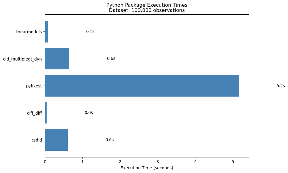
csdid Callaway & Sant'Anna 0.607066 1.704085 1.586146 0.117939 OK
diff_diff Callaway & Sant'Anna 0.049023 1.704085 1.586146 0.117939 OK
pyfixest TWFE (sunab not available) 5.165600 1.324159 1.586146 -0.261987 OK
did_multiplegt_dyn de Chaisemartin & D'Haultfoeuille (10% sample) 0.645394 1.464355 1.586146 -0.121791 OK
N/A Borusyak, Jaravel & Spiess NaN NaN NaN NaN Error: No Python implementation available
linearmodels Traditional TWFE (biased) 0.087213 1.324159 1.586146 -0.261987 OK
import matplotlib.pyplot as plt# Filter to packages with valid timestiming_data = [(r['package'], r['time']) for r in results.values()if r.get('time') isnotNone]if timing_data: packages, times =zip(*timing_data) fig, ax = plt.subplots(figsize=(10, 6)) bars = ax.barh(packages, times, color='steelblue') ax.set_xlabel('Execution Time (seconds)') ax.set_title(f'Python Package Execution Times\nDataset: {len(df):,} observations')# Add time labelsfor bar, t inzip(bars, times): ax.text(bar.get_width() +1, bar.get_y() + bar.get_height()/2,f'{t:.1f}s', va='center') plt.tight_layout() plt.show()else:print("No timing data available to plot.")
Execution time comparison (Python packages)
5.9 Python Package Availability Notes
5.9.1 Available Packages
csdid: Full implementation of Callaway & Sant’Anna
Install: pip install csdid
Supports doubly-robust estimation
Can be slow with very large datasets
diff_diff: Alternative CS implementation
Install: pip install diff-diff
Generally faster than csdid
Good for event study aggregation
pyfixest: Port of R’s fixest
Install: pip install pyfixest
Fast fixed effects estimation
Sun & Abraham support varies by version
did_multiplegt_dyn: de Chaisemartin & D’Haultfoeuille
Install: pip install did-multiplegt-dyn
Python port of the R/Stata command
Computationally intensive for large datasets
5.9.2 Not Available in Python
Missing Python Implementation
The following estimator does not have a native Python package:
Borusyak, Jaravel & Spiess (didimputation) - Only available in R and Stata - No community Python port exists
For this method, users must either:
Use R (recommended via Quarto or rpy2)
Use Stata
Implement the method from scratch
Source Code
---title: "Python Package Analysis"---# Python Packages for Staggered DiDThis chapter benchmarks Python packages for difference-in-differences with staggered treatment. Python has fewer native implementations compared to R, but several community packages exist.## Package Availability Summary| Method | R Package | Python Package | Status ||--------|-----------|----------------|--------|| Callaway & Sant'Anna | `did` | `csdid`, `diff_diff` | Available || de Chaisemartin & D'Haultfoeuille | `DIDmultiplegtDYN` | `did_multiplegt_dyn` | Available || Sun & Abraham | `fixest::sunab` | `pyfixest` | Available (partial) || Borusyak, Jaravel & Spiess | `didimputation` | None | **Not available in Python** |```{python}#| label: setup-python#| warning: falseimport numpy as npimport pandas as pdimport timeimport warningswarnings.filterwarnings('ignore')# Load the datadf = pd.read_csv("sim_data.csv")print(f"Data loaded:")print(f"Observations: {len(df):,}")print(f"Units: {df['id'].nunique():,}")print(f"Periods: {df['year'].nunique()}")# Calculate true ATT (from treated observations' true effects)# We need to regenerate true effects since CSV doesn't have themtreat_cohorts = [0, 2012, 2014, 2016, 2018]cohort_effects = {0: 0, 2012: 0.5, 2014: 0.3, 2016: 0.1, 2018: 0.0}tau_0 =1.0gamma =0.1df['tau_gt'] =0.0mask = df['treated'] ==Truedf.loc[mask, 'tau_gt'] = ( tau_0 + df.loc[mask, 'first_treat'].map(cohort_effects) + gamma * (df.loc[mask, 'year'] - df.loc[mask, 'first_treat']))true_overall_att = df.loc[df['treated'], 'tau_gt'].mean()print(f"\nTrue overall ATT: {true_overall_att:.4f}")# Store resultsresults = {}```## 1. Callaway & Sant'Anna (`csdid`)The `csdid` package is a Python port of the original R `did` package.```{python}#| label: csdid#| warning: false#| cache: truetry:from csdid.att_gt import ATTgtprint("Running csdid ATTgt()...")print("This may take several minutes with 1M units.\n") start_time = time.perf_counter() att_gt = ATTgt( yname='y', gname='first_treat', idname='id', tname='year', data=df ) out_csdid = att_gt.fit(est_method='dr') # doubly robust csdid_time = time.perf_counter() - start_timeprint(f"\nExecution time: {csdid_time:.2f} seconds")# Aggregate to dynamic effects agg_dynamic = out_csdid.aggte(typec='dynamic', na_rm=True)# Extract overall ATT from the aggregation csdid_att = agg_dynamic.summ_attgt().atte['overall_att']print(f"\nEstimated ATT: {csdid_att:.4f}"if csdid_att else"ATT not extracted")print(f"True ATT: {true_overall_att:.4f}") results['csdid'] = {'package': 'csdid','method': 'Callaway & Sant\'Anna','time': csdid_time,'att': csdid_att,'output': out_csdid }exceptImportErroras e:print("Package csdid not installed.")print("Install with: pip install csdid") results['csdid'] = {'package': 'csdid','method': 'Callaway & Sant\'Anna','time': None,'error': str(e) }exceptExceptionas e:print(f"Error running csdid: {e}") results['csdid'] = {'package': 'csdid','method': 'Callaway & Sant\'Anna','time': None,'error': str(e) }```## 2. Alternative CS Implementation (`diff_diff`)The `diff_diff` package provides another implementation of Callaway & Sant'Anna.```{python}#| label: diff-diff#| warning: false#| cache: truetry:from diff_diff import CallawaySantAnnaprint("Running diff_diff CallawaySantAnna()...")print() cs = CallawaySantAnna() start_time = time.perf_counter() cs_results = cs.fit( df, outcome='y', unit='id', time='year', first_treat='first_treat', aggregate='event_study' ) diff_diff_time = time.perf_counter() - start_timeprint(f"Execution time: {diff_diff_time:.2f} seconds")# Extract ATT from event studyifhasattr(cs_results, 'event_study_effects'): post_effects = [v['effect'] for k, v in cs_results.event_study_effects.items()if k >=0] diff_diff_att = np.mean(post_effects) if post_effects elseNoneelse: diff_diff_att =Noneprint(f"\nEstimated ATT (post-treatment avg): {diff_diff_att:.4f}"if diff_diff_att else"")print(f"True ATT: {true_overall_att:.4f}") results['diff_diff'] = {'package': 'diff_diff','method': 'Callaway & Sant\'Anna','time': diff_diff_time,'att': diff_diff_att,'output': cs_results }exceptImportErroras e:print("Package diff_diff not installed.")print("Install with: pip install diff-diff") results['diff_diff'] = {'package': 'diff_diff','method': 'Callaway & Sant\'Anna','time': None,'error': str(e) }exceptExceptionas e:print(f"Error running diff_diff: {e}") results['diff_diff'] = {'package': 'diff_diff','method': 'Callaway & Sant\'Anna','time': None,'error': str(e) }```## 3. Sun & Abraham via `pyfixest`The `pyfixest` package is a Python port of the R `fixest` package and includes support for Sun & Abraham estimation.```{python}#| label: pyfixest#| warning: false#| cache: truetry:import pyfixest as pfprint("Running pyfixest for Sun & Abraham...")print()# Prepare data for pyfixest df_pf = df.copy() df_pf['cohort'] = df_pf['first_treat'].replace(0, np.inf) # Never-treated = Inf start_time = time.perf_counter()# Sun & Abraham estimation# pyfixest uses i() for interaction-weighted estimatortry:# Try sunab-style estimation out_pf = pf.feols("y ~ sunab(cohort, year) | id + year", data=df_pf, vcov={'CRV1': 'id'} ) pf_time = time.perf_counter() - start_timeprint(f"Execution time: {pf_time:.2f} seconds")print(out_pf.summary())# Extract ATT pf_att = out_pf.coef().mean() # Average of event study coefficients results['pyfixest'] = {'package': 'pyfixest','method': 'Sun & Abraham','time': pf_time,'att': pf_att,'output': out_pf }exceptExceptionas e:# Fallback to simple TWFEprint(f"sunab not available in pyfixest, running TWFE: {e}") out_pf = pf.feols("y ~ treated | id + year", data=df_pf, vcov={'CRV1': 'id'} ) pf_time = time.perf_counter() - start_timeprint(f"\nExecution time (TWFE): {pf_time:.2f} seconds")print(out_pf.summary()) results['pyfixest'] = {'package': 'pyfixest','method': 'TWFE (sunab not available)','time': pf_time,'att': out_pf.coef()['treated'],'output': out_pf }exceptImportErroras e:print("Package pyfixest not installed.")print("Install with: pip install pyfixest") results['pyfixest'] = {'package': 'pyfixest','method': 'Sun & Abraham','time': None,'error': str(e) }exceptExceptionas e:print(f"Error running pyfixest: {e}") results['pyfixest'] = {'package': 'pyfixest','method': 'Sun & Abraham','time': None,'error': str(e) }```## 4. de Chaisemartin & D'Haultfoeuille (`did_multiplegt_dyn`)The `did_multiplegt_dyn` package is a Python port of the original Stata/R command by de Chaisemartin & D'Haultfoeuille.**Method**: Compares switchers to non-switchers at each period, robust to heterogeneous treatment effects.```{python}#| label: dcdh-python#| warning: false#| cache: trueimport polars as plfrom did_multiplegt_dyn import DidMultiplegtDynprint("Running DidMultiplegtDyn()...")print("Note: This estimator can be computationally intensive.\n")# Convert pandas DataFrame to polars and prepare datadf_dcdh = pl.from_pandas(df)df_dcdh = df_dcdh.with_columns([ pl.col('treated').cast(pl.Int32).alias('D')])start_time = time.perf_counter()try:# Create model instance model_dcdh = DidMultiplegtDyn( df=df_dcdh, outcome='y', group='id', time='year', treatment='D', effects=5, placebo=3, cluster='id' )# Fit the model model_dcdh.fit() dcdh_time = time.perf_counter() - start_time# Get summary table dcdh_summary = model_dcdh.summary()print(f"\nExecution time (10% sample): {dcdh_time:.2f} seconds")print(f"Estimated full data time: ~{dcdh_time *10:.0f} seconds")print()print(dcdh_summary)# Extract Average_Total_Effect from summary table dcdh_att = model_dcdh.result['did_multiplegt_dyn']['ATE']['Estimate'].values[0] results['did_multiplegt_dyn'] = {'package': 'did_multiplegt_dyn','method': 'de Chaisemartin & D\'Haultfoeuille (10% sample)','time': dcdh_time,'estimated_full_time': dcdh_time *10,'att': dcdh_att,'output': dcdh_summary }exceptExceptionas e:print(f"Error during estimation: {e}")import traceback traceback.print_exc() results['did_multiplegt_dyn'] = {'package': 'did_multiplegt_dyn','method': 'de Chaisemartin & D\'Haultfoeuille','time': None,'att': None,'error': str(e) }```## 5. Borusyak, Jaravel & Spiess (Imputation)::: {.callout-warning}## Not Available in PythonThere is **no native Python package** implementing the imputation estimator from Borusyak, Jaravel & Spiess. This method is only available in:- **R**: `didimputation` package- **Stata**: `did_imputation` command:::```{python}#| label: imputation-unavailableprint("="*60)print("Borusyak, Jaravel & Spiess (did_imputation)")print("="*60)print()print("STATUS: NOT AVAILABLE IN PYTHON")print()print("This estimator is only available in:")print(" - R: didimputation package")print(" - Stata: did_imputation command")print()results['didimputation'] = {'package': 'N/A','method': 'Borusyak, Jaravel & Spiess','time': None,'att': None,'error': 'No Python implementation available'}```## 6. Traditional TWFE (Biased Baseline)For comparison, let's run traditional TWFE using `linearmodels` or `statsmodels`:```{python}#| label: twfe-python#| warning: false#| cache: truetry:from linearmodels.panel import PanelOLSprint("Running traditional TWFE with linearmodels...")print()# Prepare panel data structure df_panel = df.set_index(['id', 'year']) start_time = time.perf_counter() model = PanelOLS( df_panel['y'], df_panel[['treated']].astype(float), entity_effects=True, time_effects=True ) out_twfe = model.fit(cov_type='clustered', cluster_entity=True) twfe_time = time.perf_counter() - start_timeprint(f"Execution time: {twfe_time:.2f} seconds")print(out_twfe.summary.tables[1]) twfe_att = out_twfe.params['treated']print(f"\nTWFE ATT estimate: {twfe_att:.4f}")print(f"True ATT: {true_overall_att:.4f}")print(f"Bias: {twfe_att - true_overall_att:.4f}") results['twfe_linearmodels'] = {'package': 'linearmodels','method': 'Traditional TWFE (biased)','time': twfe_time,'att': twfe_att,'output': out_twfe }exceptImportError:print("Package linearmodels not installed.")print("Install with: pip install linearmodels")# Fallback to statsmodelstry:import statsmodels.api as smfrom statsmodels.regression.linear_model import OLSprint("\nRunning TWFE with statsmodels (demeaned)...")# Demean for fixed effects df_fe = df.copy() df_fe['y_demeaned'] = df_fe.groupby('id')['y'].transform(lambda x: x - x.mean()) df_fe['y_demeaned'] = df_fe.groupby('year')['y_demeaned'].transform(lambda x: x - x.mean()) df_fe['treated_demeaned'] = df_fe.groupby('id')['treated'].transform(lambda x: x - x.mean()) df_fe['treated_demeaned'] = df_fe.groupby('year')['treated_demeaned'].transform(lambda x: x - x.mean()) start_time = time.perf_counter() model = OLS(df_fe['y_demeaned'], df_fe['treated_demeaned']).fit() twfe_time = time.perf_counter() - start_timeprint(f"Execution time: {twfe_time:.2f} seconds")print(f"TWFE ATT: {model.params[0]:.4f}") results['twfe_statsmodels'] = {'package': 'statsmodels','method': 'Traditional TWFE (biased)','time': twfe_time,'att': model.params[0] }exceptExceptionas e:print(f"Error: {e}")exceptExceptionas e:print(f"Error running TWFE: {e}")```## Python Results Summary```{python}#| label: python-summaryimport pandas as pd# Create summary tablesummary_data = []for name, r in results.items(): summary_data.append({'Package': r.get('package', 'N/A'),'Method': r.get('method', 'N/A'),'Time (s)': r.get('time'),'ATT': r.get('att'),'True ATT': true_overall_att if r.get('time') elseNone,'Bias': (r.get('att') - true_overall_att) if r.get('att') elseNone,'Status': 'Error: '+ r.get('error', '') if r.get('error') else'OK' })summary_df = pd.DataFrame(summary_data)print("\n"+"="*80)print("PYTHON PACKAGE COMPARISON SUMMARY")print("="*80)print(summary_df.to_string(index=False))# Save for comparison chaptersummary_df.to_csv("python_results.csv", index=False)``````{python}#| label: python-timing-plot#| fig-cap: "Execution time comparison (Python packages)"import matplotlib.pyplot as plt# Filter to packages with valid timestiming_data = [(r['package'], r['time']) for r in results.values()if r.get('time') isnotNone]if timing_data: packages, times =zip(*timing_data) fig, ax = plt.subplots(figsize=(10, 6)) bars = ax.barh(packages, times, color='steelblue') ax.set_xlabel('Execution Time (seconds)') ax.set_title(f'Python Package Execution Times\nDataset: {len(df):,} observations')# Add time labelsfor bar, t inzip(bars, times): ax.text(bar.get_width() +1, bar.get_y() + bar.get_height()/2,f'{t:.1f}s', va='center') plt.tight_layout() plt.show()else:print("No timing data available to plot.")```## Python Package Availability Notes### Available Packages1. **`csdid`**: Full implementation of Callaway & Sant'Anna - Install: `pip install csdid` - Supports doubly-robust estimation - Can be slow with very large datasets2. **`diff_diff`**: Alternative CS implementation - Install: `pip install diff-diff` - Generally faster than `csdid` - Good for event study aggregation3. **`pyfixest`**: Port of R's fixest - Install: `pip install pyfixest` - Fast fixed effects estimation - Sun & Abraham support varies by version4. **`did_multiplegt_dyn`**: de Chaisemartin & D'Haultfoeuille - Install: `pip install did-multiplegt-dyn` - Python port of the R/Stata command - Computationally intensive for large datasets### Not Available in Python::: {.callout-important}## Missing Python ImplementationThe following estimator does **not have a native Python package**:**Borusyak, Jaravel & Spiess** (`didimputation`) - Only available in R and Stata - No community Python port existsFor this method, users must either:- Use R (recommended via Quarto or rpy2)- Use Stata- Implement the method from scratch:::